A Basic Introduction to Quantum GANs

“Quantum computing just becomes vastly simpler once you take the physics out of it.”

As quantum hardware advances, there is potential for a quantum advantage in specialized data-generating tasks, potentially exceeding classical approaches. Quantum Generative Adversarial Networks (QGANs) are a promising advancement in synthetic data generation, particularly for tabular data.

Quantum circuits: the universal language of quantum computing

As I recall Scott Aaronson remark, quantum computing just becomes vastly simpler once you take the physics out of it. We use quantum circuits that are like recipes or instruction manuals for quantum computers. They describe, step by step, what operations to perform on qubits (the quantum version of classical bits) to carry out a quantum computation. These circuits are capable of representing and manipulating complex probability distributions that classical neural networks may struggle with. This could result in more accurate modeling of complex patterns and correlations in tabular data. In general, quantum systems can effectively represent and handle multidimensional data. For tabular datasets with a large number of features, this could result in more compact and robust models. These systems have inherent randomness, which may be useful in generating diverse and realistic synthetic samples, thus boosting the overall quality and diversity of the generated data. The probabilistic nature of quantum measurements may provide additional levels of privacy protection in synthetic data generation, which is critical for sensitive tabular data.

Quantum circuits inherently integrate non-linear transformations, which may be useful in capturing complex, non-linear relationships that exist in real-world tabular data. Some quantum algorithms provide quadratic speedups over their classical equivalents. While not certain, the ability to train and generate big datasets more quickly could be significant. Moreover Quantum circuits may provide unique approaches to handling categorical variables in tabular data, potentially resulting in more natural or effective encoding.

While these potential benefits are exciting, it’s important to remember that quantum machine learning, including QGANs, is still in its early stages. The limitations of current quantum technology are often present in implementations that use hybrid quantum-classical techniques.

Note: Don't let the terminology used in quantum computing overwhelm you. It’s just a matter of understanding that in the quantum world there are a number of axioms that are different from those of classical physics. You can find some very entertaining explanations on the Pennylane website (which is the library we’re going to use in our example). If you want more detail, one of the reference books on the subject is Quantum Computation and Quantum Information by Nielsen and Chuang.

Quantum generator

Now, let us integrate this information into our proposal on the Tabular Quantum GAN (TQG). We can introduce this concept after explaining the fundamental quantum concepts and before getting into the specific implementation:

In our Tabular Quantum GAN (TQG), quantum circuits act as an essential component of our generator. But what precisely are quantum circuits, and why do they matter? Sit tight for a second: I just mentioned quantum generators, and GANs include discriminators as well.

The purpose of the generator is to produce new, fake data samples. The special features of quantum systems, such as entanglement and superposition, can greatly aid in this task. Compared to conventional generators, quantum ones may be able to scour the data space more quickly and pick up on complex patterns.The discriminator’s job is to figure out if data is real or fake. This is simply a binary classification problem, which conventional machine learning approaches are already proficient at addressing.

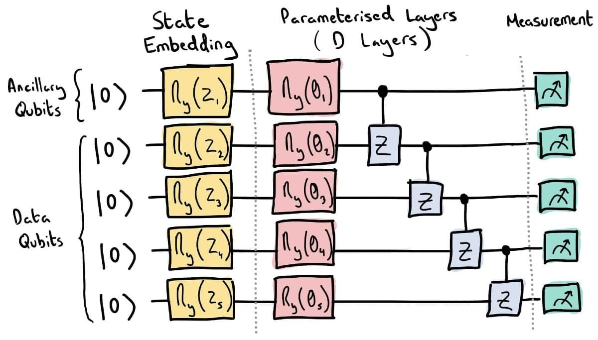
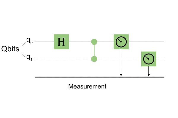
Now we can follow with the TGAN. As previously stated, quantum circuits are the primary form of communication with quantum computers or quantum simulators. Quantum circuits define operations for quantum computers in the same way that programming languages such as Python do for classical computers. Consider a quantum circuit as a blueprint for quantum computation: Our ingredients are qubits, the quantum equivalent of classical bits. The steps in our recipe represent quantum gates, which are operations performed on these qubits.

At the end of our process, we take measurements to obtain our results, turning quantum information into classical information that we can understand and apply.

In our TQG implementation, we use PennyLane, a software framework for describing quantum circuits. When we run our code, PennyLane translates the circuit descriptions into operations that can be executed on a quantum simulator. As quantum hardware becomes more accessible, the identical circuit specifications may be communicated to genuine quantum computers.

Here’s a simplified version of how our quantum circuit is defined in Python code:

## This code is inspired in an example from Pennylane library's page,  
## authored by James Ellis. You can find this example here:  
## https://pennylane.ai/qml/demos/tutorial_quantum_gans/ 
 
@qml.qnode(dev, diff_method="parameter-shift") 
def quantum_circuit(noise, weights): 
    weights = weights.reshape(q_depth, n_qubits) 
    # Initialize qubits 
    for i in range(n_qubits): 
        qml.RY(noise[i], wires=i) 
 
    # Apply quantum operations 
    for i in range(q_depth): 
        for y in range(n_qubits): 
            qml.RY(weights[i][y], wires=y) 
        for y in range(n_qubits - 1): 
            qml.CZ(wires=[y, y + 1]) 
 
    # Measure the results 
    return qml.probs(wires=list(range(n_qubits))) 
 
def partial_measure(noise, weights): 
    # Non-linear Transform 
    probs = quantum_circuit(noise, weights) 
    probsgiven0 = probs[: (2 ** (n_qubits - n_a_qubits))] 
    probsgiven0 /= tf.reduce_sum(probs) 
 
    # Post-Processing 
    probsgiven = probsgiven0 / tf.reduce_max(probsgiven0) 
    return probsgiven

This quantum circuit function defines the operations performed on our
qubits. Let’s break it down:

1. Function Decorator

@qml.qnode(dev, diff_method="parameter-shift")

This decorator turns our Python function into a quantum node (qnode)
in PennyLane. It specifies that the circuit should run on the quantum device ‘dev’ (that we have already selected). diff_method=”parameter-shift”’ indicates the method used to compute gradients of the circuit, necessary for training.

2. Function Inputs

def quantum_circuit(noise, weights):

In this function, ‘noise’: is an n array of values used to initialize the qubits, and ‘weights’ is a 2D array of parameters for the quantum operations.

3. Weights reshape

weights = weights.reshape(q_depth, n_qubits)

Reshaping the weights will be important for building the GAN.

4. Qubit Initialization

for i in range(n_qubits): 
    qml.RY(noise[i], wires=i)

Mathematically, RY can be expressed as a unitary matrix:

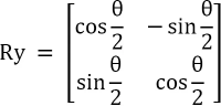
This loop applies an RY (rotation around Y-axis) gate to each qubit. The rotation angle in the matrix for each qubit is specified by the corresponding ‘noise’ value. This initializes each qubit in a specific quantum state.

5. Quantum Operations

# Apply quantum operations 
    for i in range(q_depth): 
        for y in range(n_qubits): 
            qml.RY(weights[i][y], wires=y) 
        for y in range(n_qubits - 1): 
            qml.CZ(wires=[y, y + 1])

This nested loop structure applies a series of quantum operations ‘q_depth’ times. In each iteration, an RY rotation is applied to each qubit, with angles specified by ‘weights’. CZ (controlled-Z) gates are applied between adjacent qubits. This creates entanglement between qubits and allows for complex quantum states.

6. Measurement

return qml.probs(wires=list(range(n_qubits)))

Finally, this returns the probabilities of measuring each possible state of the qubits. For n qubits, this gives 2^n probability values.

This circuit’s structure creates complex quantum states that can represent and generate complex patterns in data. The alternating RY and CZ gates create a balance of single-qubit rotations and two-qubit entanglements, which is determinant for the expressiveness of the quantum circuit.

7. Partial measurement

def partial_measure(noise, weights):

This function performs a partial measurement on our quantum circuit and post-processes the results. This function has to inputs: ‘noise’ and ‘weights’.

— ‘noise’: The same noise input used in the quantum_circuit function. — ‘weights’: The trainable parameters of our quantum circuit.

probs = quantum_circuit(noise, weights)

This part performs a Non-linear Transformation calling our quantum circuit and getting the probability distribution of all possible qubit states.

probsgiven0 = probs[: (2 ** (n_qubits - n_a_qubits))]

This line slices the probability distribution to keep only the first 2^(n_qubits — n_a_qubits) probabilities, and is equivalent to measuring only (n_qubits — n_a_qubits) qubits and leaving n_a_qubits unmeasured.

probsgiven0 /= tf.reduce_sum(probs) 
probsgiven = probsgiven0 / tf.reduce_max(probsgiven0)

This first line normalizes the probabilities by dividing by the sum of all probabilities, ensuring that our partial measurement results still form a valid probability distribution. The second line divides all probabilities by the maximum probability in the distribution. This operation scales the probabilities to be between 0 and 1, with at least one probability equal to 1.

Finally, the function returns the post-processed partial measurement results. The partial_measure function is critical :

1. Introduce non-linearity into our quantum operations, which is important for the expressiveness of our model.
2. Control the dimensionality of our output, making it easier to interface with classical neural network layers.
3. Ensure our output is properly normalized and scaled, which can help with the stability and effectiveness of our GAN training process.

Now we can build our generator:

# Quantum generator 
class PatchQuantumGenerator(nn.Module): 
    """Quantum generator class for the patch method""" 
 
    def __init__(self, n_generators, output_dim, q_delta=1): 
        super().__init__() 
 
        self.q_params = nn.ParameterList( 
            [nn.Parameter(q_delta * torch.rand(q_depth * n_qubits), requires_grad=True) for _ in range(n_generators)] 
        ) 
        self.n_generators = n_generators 
        self.output_dim = output_dim 
 
    def forward(self, x): 
        patch_size = 2 ** (n_qubits - n_a_qubits) 
        total_patches = (self.output_dim + patch_size - 1) // patch_size  # Total number of patches needed 
        fake = torch.Tensor(x.size(0), 0).to(device) 
 
        for params in self.q_params: 
            patches = torch.Tensor(0, patch_size).to(device) 
 
            for elem in x: 
                q_out = partial_measure(elem, params).float().unsqueeze(0) 
                patches = torch.cat((patches, q_out)) 
 
            fake = torch.cat((fake, patches), 1) 
 
        fake = fake[:, :self.output_dim]  # Ensure the output dimension matches exactly 
        return fake

Train the GAN

Once we have defined our generator, we can train the GAN in the “classical” way. In the below code, the training loop implements the adversarial process characteristic of GANs. The discriminator is trained on both real and fake (generated) data. The generator is trained to fool the discriminator. The process alternates between improving the discriminator and the generator. We have used binary cross-entropy loss, which is typical for GANs. The quantum circuit then processes the generator's input, which is random noise.

# Generate the same number of samples than input data 
input_dim = data.shape[1] 
 
#Learning rates 
lrG = 0.0001 
lrD = 0.0001 
 
num_iter = 300 
 
discriminator = Discriminator(input_dim).to(device) 
generator = PatchQuantumGenerator(n_generators, input_dim).to(device) 
 
criterion = nn.BCELoss() 
# Use optimizers like Adam or RMSProp with adaptive learning 
# rates to ensure more stable training. 
# To do: Implement learning rate scheduling to reduce the learning rate 
#as training progresses, which helps in converging to better solutions. 
optD = optim.Adam(discriminator.parameters(), lr=lrD) 
optG = optim.Adam(generator.parameters(), lr=lrG) 
 
real_labels = torch.full((batch_size,), 1.0, dtype=torch.float, device=device) 
fake_labels = torch.full((batch_size,), 0.0, dtype=torch.float, device=device) 
 
counter = 0 
 
while True: 
    for i, (data, _) in enumerate(dataloader): 
        real_data = data.to(device) 
        noise = torch.rand(batch_size, n_qubits, device=device) * math.pi / 2 
        fake_data = generator(noise) 
 
        discriminator.zero_grad() 
        outD_real = discriminator(real_data).view(-1) 
        outD_fake = discriminator(fake_data.detach()).view(-1) 
 
        errD_real = criterion(outD_real, real_labels) 
        errD_fake = criterion(outD_fake, fake_labels) 
        errD_real.backward() 
        errD_fake.backward() 
        errD = (errD_real + errD_fake)/2 
        optD.step() 
 
        generator.zero_grad() 
        outD_fake = discriminator(fake_data).view(-1) 
        errG = criterion(outD_fake, real_labels) 
        errG.backward() 
        optG.step() 
 
        counter += 1 
 
        if counter % 20 == 0: 
            print(f'Iteration: {counter}, Discriminator Loss: {errD:0.3f}, Generator Loss: {errG:0.3f}') 
 
        if counter == num_iter: 
            break 
 
    if counter == num_iter: 
        break

Experiment results

We are going to make a simple experiment using the dataset 'make-circles’ that we can find in the Scikitlearn library (Authors: B. Thirion, G. Varoquaux, A. Gramfort, V. Michel, O. Grisel, G. Louppe, J. Nothman; License: BSD 3 clause). The results can be seen in the following figure.

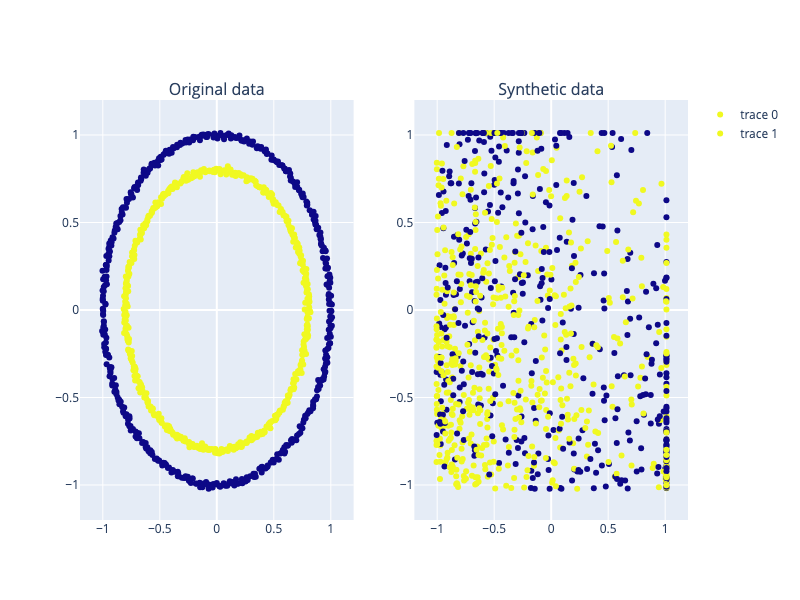
To be honest, the two figures don’t look too similar at first glance. However, when using some metrics to compare the synthetic data with the original, the result is excellent:

"""Cluster Analysis Measure (Woo et al. 2009) 
Large Uc values indicate disparities in the cluster 
memberships, which in turn suggest differences in the 
distributions of the original and masked data. 
References: 
Woo M.-J., Reiter J. P., Oganian A., Karr A. F. Global 
Measures of Data Utility for Microdata Masked for Disclosure 
Limitation. J. Priv Confidentiality. 2009;1(1):111–24.""" 
Cluster measure = -0.11 
 
"""Propensity score method 
Propensity score mean-squared error pMSE (Woo et al. 2009). If 
a ratio score of 0 implies the two datasets are identical. A 
score of 1 implies that are totally different. 
 
References: 
Woo M.-J., Reiter J. P., Oganian A., Karr A. F. Global 
Measures of Data Utility for Microdata Masked for Disclosure 
Limitation. J Priv Confidentiality. 2009;1(1):111–24.""" 
Propensity score mean-squared error pMSE = 0.0097 
 
Synthetic data similarity = 99.03%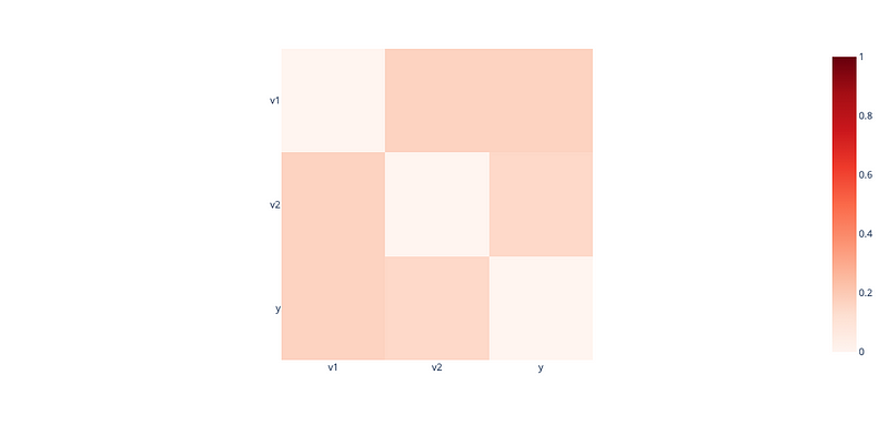

Conclusions

It was not my intention to write a post in which I stated that “this method outperforms existing techniques” or something similar. My goal was merely to show the potential uses of quantum computing in synthetic data generation. GANs are fascinating algorithms with lots of possibilities. Synthetic data generation is certainly a trendy issue today. You can find the notebook in which I ran the experiment here. Perhaps the “quantum” generator that I used in the experiment was the simplest one I could use. To achieve better results, I encourage you to experiment with other generator setups (some of which are suggested in the notebook). Finally, I’d want to point out that I didn’t go into detail regarding the quantum physics axioms that base quantum computing. I am not an expert on the issue, nor was that the purpose of this writing.