A Story of Long Tails

“Details matter. It’s worth waiting to get it right.”
Steve Jobs

Those of us who have made MMM models using Bayesian hierarchical models have seen that these models¹ provide lots of information about each of the parameters we set up in the model. By applying rigorous and widely validated statistical techniques, we choose, for example, the mean (sometimes the median) of the posterior distribution as the value of the influence for a certain channel. Then, we consider and generate actionable insights from this value. However, the truth is that Bayesian analysis gives us as output a probability distribution of values, and the tails are frequently large with rare occurrences and exceptions. If we underestimate the information contented in these tails, we are losing a valuable opportunity. In the expression of those long tails, if we look with the proper lens, we can find very valuable insights. Actually, the basic idea for which most users use MMM models is to quantify the influence of each channel in, for example, monthly sales or the number of units sold. However, this is only the beginning. These models have much more to say.

► This post strives to explain where these exceptions forming the long tails come from and what they might mean using complex systems theory formalisms as the lens to look at MMM models.

"… but still there were few things to be said."

Death in the Afternoon, Ernest Hemingway

Uncertainty in Marketing Mix Modelling: the Gaussian average

One of the most important parameters to estimate in a MMM is the channel influence or effect in a given KPI (our dependent variable). This parameter is pivotal for many advertising strategies. Most quantitative MMM analyses suppose Gaussian (normal) distributions with finite means and variances [4]. This is especially important when we work with Bayesian methods for MMM [23]. In these methods, we try to infer the probability distribution (posterior) of these parameters (channel influence, lag, carryover, etc.) from the observed data using a preset “guiding” distribution (prior). Then we treat the inferred distribution according to Gaussian rules, and we choose the mean of this distribution as the statistically significant value for each of these parameters.

Nevertheless, reality is stubborn and very often (most of the time) shows rare occurrences and exceptions, what in distribution curves is known as long tails [3].

Power laws and complex systems

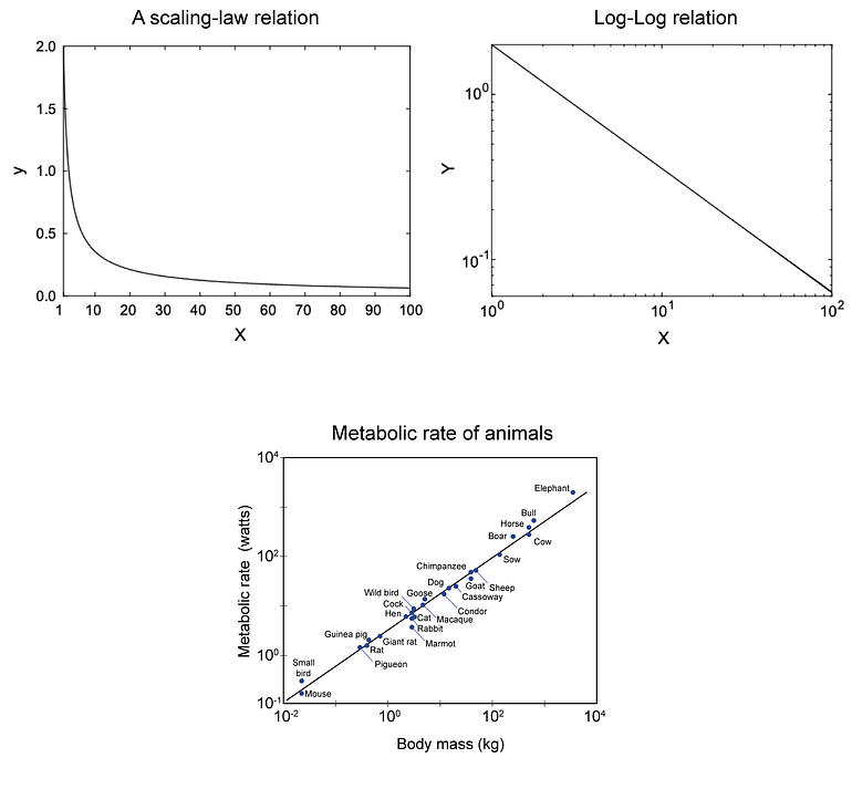
The empirical investigation of complex systems in the real world has shown a hidden pattern that holds true in a wide range of situations [18]. Power laws or scaling laws can be seen as laws of nature describing complex systems [12][30]. We call them scaling laws because they maintain their proportions regardless of scale. A scaling law is a functional relationship that relies on a polynomial with a scaling parameter α and a constant C.

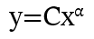
Therefore, y always changes as a power of x, and a relative change in x leads to a proportional relative change in y despite their initial values. This law is widespread in nature in a wide range of phenomena, like the size of earthquakes, the number of heartbeats of mammals in relation to their weight, or the empirical wealth distribution in the US. And yes, it is also shown in the performance of marketing channels.

Let’s consider a digital campaign in a given channel: a few posts get massive engagement (the head). Many posts get moderate engagement (the body). But most posts get minimal engagement (the tail). This behavior follows a scaling law, and this pattern is natural and can be expected. It will contain valuable information and will repeat at different scales. In the conventional MMM approach, we try to reduce variance and focus on averages. But we could decide to recognize that this variance follows predictable patterns and use this information to our benefit.

When we observe channel influence in MMM, we calculate its influence using the mean μ, representing the average effect we are going to consider for future planning decisions. The standard deviation, σ, represents the uncertainty, and the ratio σ/μ often increases with μ. This suggests a scaling law where larger effects have proportionally larger variations. The pattern repeats at different advertising investment levels. We call it scale-free behavior.

Self-organized criticality systems

In statistical mechanics, the theory of self-organized criticality (SOC) unifies power-law behavior observed in complex systems [22][27][28]. The basic idea behind SOC is that a complex system will naturally organize itself into a state that is on a critical point that is the edge of two different regimes, without intervention from outside the system [33]. This is known as a phase transition state because a system moves from one regime to another once it has reached a critical point. In the sand pile example in Figure 3, the pile will grow until a certain height (critical point). Beyond this point, the pile is not growing anymore, and the sand will start to roll down, starting a different avanlanche dynamics. This illustrates the phase transition concept.

Highly optimized tolerance mechanism

This natural organization occurs in complex systems consisting of many interacting components, as in the case of the sand pile. The mechanism is known as highly optimized tolerance (HOT). Most complex systems consist of many heterogeneous components, which often have a complex structure and behavior of their own. The interaction of these components forms a large and more robust system with a specific behavior [8]. It’s like showing a global dynamics that is the result of the interaction of multiple different dynamics. This system's dynamics represent the optimal one that captures all the dynamics that build the system.

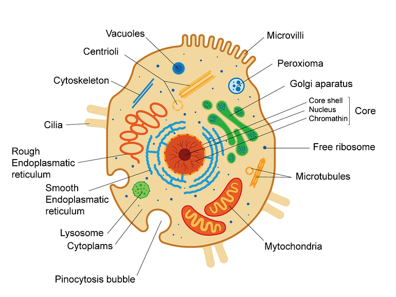
In media advertising, multiple factors or mechanisms, such as different audiences, contexts, touchpoints, or seasonality effects, contribute to the wide range of responses or long tails observed in advertising channel effectiveness modelling. All these effects have complex dynamics of their own, like, for example, the complex social influence effect on audiences or the network effect. This mechanism's diversity makes the channel influence (global optimal mechanism) more robust, just like the different cell’s components perform different specialized functions in Figure 4. This behavior is reflected in the long tails of the probability distribution of a channel influence. This influence value clusters around an average, but we also get “specialized” mechanisms represented by points distant to the main corpus of values (the long tails). These unusual responses or exceptions are the channel’s mechanism key for adapting the system (channel influence) to different situations in an optimal way. In other words, without these long tails, the channel influence could not be optimal.

System properties

The most important takeaway is that channel influence long tails don’t just happen when similar effects interact and add up. This is called self-similarity, and it is a property of systems that have similar structures at different scales [7]. When different mechanisms (let's call them sub-systems) interact with each other, we call it self-dissimilarity. The concepts of self-similarity and self-dissimilarity are important for advertising. When our advertising campaign as a system shows self-similarity (in the inner mechanisms), it could be understood as a very effective system. The contrary could mean that we have very different mechanisms that perform with less effectiveness, but its diversity can offer several other advantages.

► What is important to take into account is that high uncertainty in channel influence isn’t a problem with the measurement or a statistical reality; it’s an indicator of a robust, optimal complex system made up of diverse mechanisms that work together.

Percolation

An important concept from statistical mechanics is the percolation mechanism [19]. Think about how water flows through different types of surfaces. In a random, porous material like a sponge, water spreads pretty evenly in all directions. But we can also design an irrigation system for a garden to bring water accurately where it is needed. This will not be a random system because main channels and smaller branches have been specifically designed to reach specific points while being efficient with water. This design works as a HOT system. Marketing channels work similarly. In some cases, like a viral social media campaign, information might spread somewhat randomly through the network. But when we accurately design a marketing campaign, the spread of influence follows optimized paths, like in the irrigation system. This is where the parameter 𝛾 enters into play. For lower levels, the channel behaves more like our sponge—information spreads relatively randomly through the audience network. But higher levels represent a behaviour more like our irrigation system. Some pathways become super-efficient (like main irrigation channels), while others serve as backups or reach specific audience segments (like smaller irrigation branches). This optimization naturally creates long tails in our channel influence distribution, proving that the channel is well-optimized and robust.

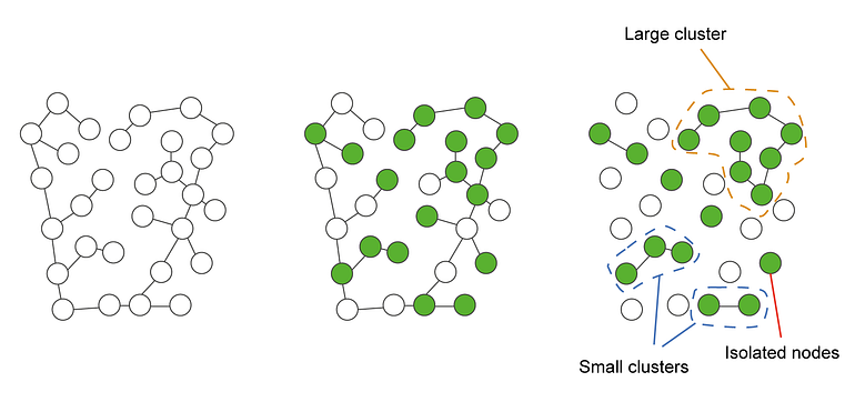
Marketing researchers have already studied percolation for product diffusion mechanisms. Figure 6 represents the percolation in a network of consumers considering whether to buy a new product with a given quality, Q ∈ [0, 1]. When the product is launched, the consumer has a quality expectation q ∈ [0, 1]. Only consumers with Q > q are willing-to-buy (green nodes), while the others are not (empty nodes). Finally, consumers that are not willing to buy are removed from the networks, and their links are removed as well. This process can lead to the formation of clusters of consumers. These clusters can have different sizes, and we can also find isolated nodes without any connection. If a cluster is sufficiently large, consumers act as a single body or group.

The consumer response curve

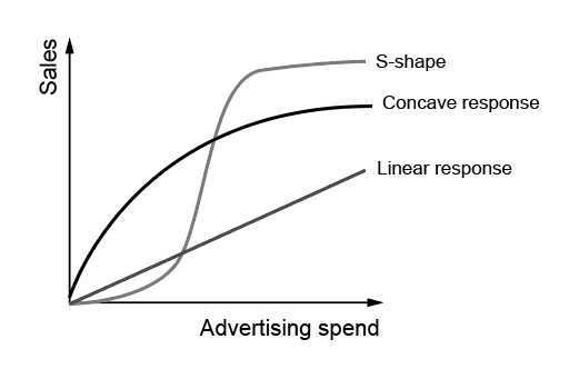
The consumer response curve is an important part of the MMM analysis. This curve shows the incrementality of advertising channel influence when increasing the spend. Consumer response curves are mainly used to find a “saturation point” in advertising spend. It’s very common to hear expressions like “the channel is saturated” or “the audience is saturated”, but the reality is that neither the audience nor the channel saturates; it's the complex system that arrives at a critical point. This curve has its roots in classic econometric literature and semi-empirical work. Demand curves and demand elasticity belong to the field of econometry since a century ago [24][31][32][34]. In the two last decades, there has appeared more specific research considering the consumer response to advertising a different reality, especially since digital channels emerged [9][10][13][14]. The discussion about understanding the consumer response to advertising spend curve has been centered on deciding the curve shape.

► Semi-empirical work around this topic is generous and is based on the hypothesis that several effects, such as consumer fatigue to the same message, make this curve reach saturation [15].

One of the most common approaches to modeling these curves today is the Hill model [20], which has its roots in medicine. Hill’s model is widely used today, and we can find it in relevant MMM projects like Meta’s Robyn or in Google’s libraries, LighweghtMMM, or their newly released Meridian project. In my latest work about this topic [26], I introduced a different equation to model the response curve based on the theory of complex systems, scaling laws, and symmetries. This work considers the formal dynamics of complex systems and statistical mechanics principles to approach the problem. The rationale behind this work was the same question heading this post: what if we integrate rare occurrences and exceptions obtained in MMM using other well-known phenomena in nature?

Complex systems-based equation for consumer response

To model these consumer response curves, I proposed the following expression:

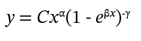
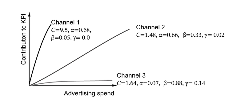
In this equation, 𝐶 is a constant reflecting the overall effectiveness of the advertising campaign, 𝛼 is the scaling parameter characterizing the relationship between consumer response and advertising spend, and 𝛽 represents the rate of change in consumer response with respect to advertising spend. Negative values suggest that the curve does not have a saturation point; alternatively, if such a point exists (near-zero 𝛽 values), it would correspond to ad spending significantly higher than the current levels. The parameter 𝛾 is the critical exponent that captures the behavior near a phase transition in consumer response and is equivalent to the percolation mechanism.

Higher 𝛼 means a stronger response to marketing input because it amplifies the effect of multiple mechanisms. For example, reaching different audiences or working in different contexts like countries, regions, seasons, or competitors efforts. With more mechanisms involved in the response, we have a higher probability of tail events, thus creating a more robust channel influence system. As 𝛾 captures the collective behavior of consumers and group dynamics, higher 𝛾 values will indicate stronger network effects. Lower values will show that we are reaching multiple small audiences, while high values show that our audience is more uniform even if it consists of the interaction of multiple audiences (similar to the percolation mechanism).

There is no direct relation between channel influence mean value and these parameters. The only significant correlation will be between channels with high 𝐶 and 𝛼 levels and high channel influence. We could say that 𝐶 is the intrinsic effectiveness of the channel, 𝛼 denotes how well we are doing in each campaign (message, segmentation, etc.); 𝛽 tells us if we are going to find a saturation point where the profitability decreases, and 𝛾 is giving us many insights about our audience (if we are reaching dispersed audiences or if we are reaching a large interconnected audience). A more comprehensive explanation of these parameters can be found in the paper [26].

► Though, recovering the aim of this post, we can link some aspects of this equation with the long tails in the channel influence distribution. The equation reflects the HOT mechanism, considering multiple mechanisms as a direct response Cxᵅ (scaling law), a saturation effect 𝛽 (global critical point with phase transition), and a collective behavior driven by 𝛾 (percolation process). Each one is highly specialized and presents a self-dissimilarity, that is, describes very different mechanisms. Different mechanisms operate at different scales, handling specific aspects and creating a more robust complex system.

Quick reference to understand channel parameters (see Appendix 1)

α — Marketing Sensitivity Index

• Range: 0 to 1
• High values (>0.5): Complex, multiple mechanisms
• Low values (<0.2): Simple, focused mechanisms
• What it tells you: Channel’s ability to scale impact with spend

β — Response Sensitivity

• Range: 0 to 1
• High values (>0.8): Rapid phase transitions, clear saturation
• Low values (<0.2): Gradual changes, no clear saturation
• What it tells you: How quickly channel reaches diminishing returns

γ — Behavioral Sensitivity Index

• Range: 0 to 1
• High values (>0.8): Strong network effects, unified audience
• Low values (<0.2): Fragmented audience, independent responses
• What it tells you: Audience clustering and viral potential

High α + High γ

• Interpretation: Complex channel with strong network effects
• Best for: Viral campaigns, broad reach

High α + Low γ

• Interpretation: Complex channel with fragmented audience
• Best for: Targeted campaigns, diversified messaging

Low α + High γ

• Interpretation: Focused channel with unified audience
• Best for: Precision targeting, community building

A brief in Bayesian inference in MMM

Point estimates in traditional Bayesian methods are based on the mean of the posterior distribution. This minimizes the expected squared error and is smooth to work with mathematically. We use the well-known Bayes theorem to calculate the posterior distribution once we define the prior distribution and get the observed data [17].

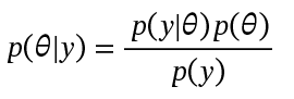
This theorem provides a specific and stable number for the channel influence (or any other variable included in the model). This has practical implications as it simplifies the management of this variable in planning scenarios [11]. However, focusing only on the mean can ignore relevant information. The long tails in posterior distributions reveal that advertising channels have potential for outsized impact, having a significant probability of higher influence. The uncertainty isn’t symmetric (more upside than downside). From a rigorous statistical perspective, using the full distribution (including tails) is actually more correct than relying on the mean (or the median) because it captures all available information and accepts asymmetric uncertainty, aligning with the original Bayesian principles of full posterior inference [5].

Bayesian inference and HOT mechanisms

The emergence of long tails in the posterior distribution aligns with the highly optimized tolerance mechanism (HOT). As we have already explained, in HOT systems, different mechanisms create robustness by interacting non-linearly, resulting in power-law distributions. In Bayesian analysis, posterior distributions often show heavy tails (most of the time if we have a sufficiently large number of samples). These multiple mechanisms appear in the likelihood, and their interactions are captured in the joint posterior. The parallel lies in how multiple mechanisms create complex distributions, not in simple variance addition. For a marketing channel with multiple mechanisms, the Bayes method can be described by the law of total probability for continuous variables:

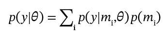
This equation calculated the total probability over discrete mechanisms, where each mechanism contributes additively and the total probability sum equals one. This can be seen as the traditional mixture model approach. Replacing the term p(y|θ) in the Bayes equation allows different mechanisms to contribute to the likelihood.

A real experiment

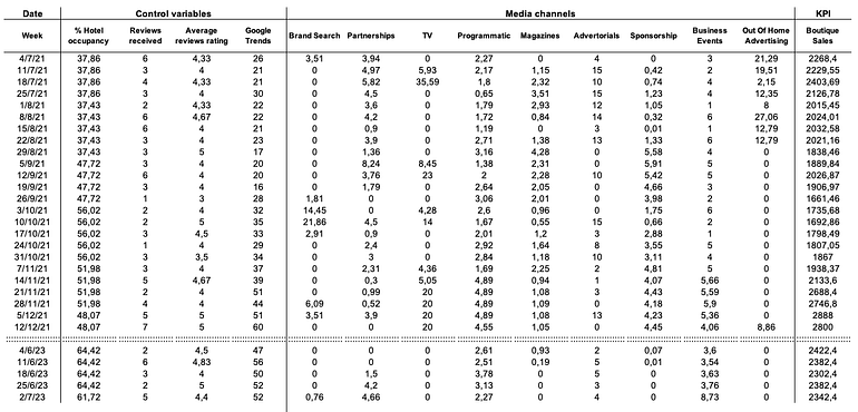
If we want to see all these concepts in practice, we can use a MMM analysis to better contextualize them. We have used a dummy dataset that simulates the advertising investment of a fashion boutique located in a European capital. This dataset includes diverse channel spend columns (both online and offline), some control variables, and a KPI column. For MMM analysis, we use the Python library LightweightMMM.

Experiment data

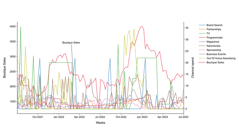
For our experiment, we have used the dummy dataset shown in Figure 9. This dataset contains weekly data of a KPI, in this case ‘Boutique Sales’, together with several media channels and control variables (non-media information). We are going to perform the experiment using both media and control variables, but we are going to focus only on the media data.

Model parameters

We started introducing our prior belief about channel influence. I have chosen a half-normal distribution with scale = 3. This choice is important because this prior only allows positive influence values with support [0,∞) making sense in a business context (we assume a channel can not negatively influence a KPI). A scale value of 3 allows for reasonable effect sizes; that is, we are holding rare occurences and exceptions with a natural tail behavior. If we consider lower scale values, we could be adding a constraint to the model to ignore rare events.

LightweightMMM uses MCMC as a sampling process [29]. The model collects thousands of samples of possible channel influence values, creating posterior distributions that often show long tails. These tails represent real uncertainty and thus additional information about channel performance. Long tails in the posterior can emerge from several mechanisms, like the appearance of multiplicative effects. When combining likelihood and prior in log space, multiplicative effects become additive, preserving and potentially amplifying tail behavior. The Hamiltonian Monte Carlo explores the full posterior, including low-probability but high-impact regions. The NUTS sampler used in Lightweight MMM operates with an unnormalized posterior because sampling doesn't require normalizing the constant p(y).

To prepare the data, we have used the scalers available in the library. To fit the model, we have used the following parametrization:

mmm, model = fit_model(
  media_data_train=media_data_train,
  target_train=target_train,
  extra_features=extra_features,
  costs=costs,
  model_name='carryover',
  seasonality_degrees=4,
  acceptance_p=0.85,
  number_warmup=2000,
  samples=2000
  )

We have chosen the ‘carryover’ model with 4 degrees of seasonality because we have weekly data. We are working with 2000 samples of posterior to get a more realistic result.

Results

Part 1: Complex systems and Power Laws

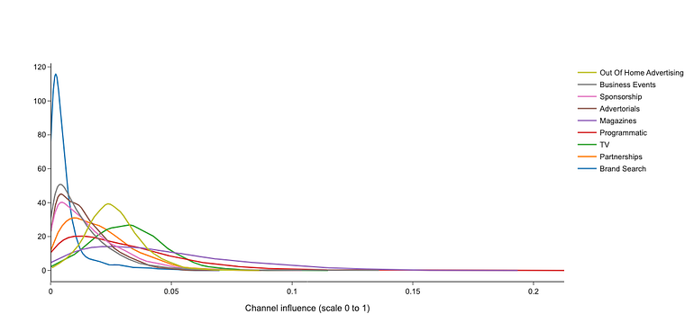
Figure 11 shows the distributions of channel influences as a result of the model. The long tails in posterior distributions indicate that advertising channels have potential for outsized impact, having a significant probability of higher influence. The uncertainty isn’t symmetric as we expected.

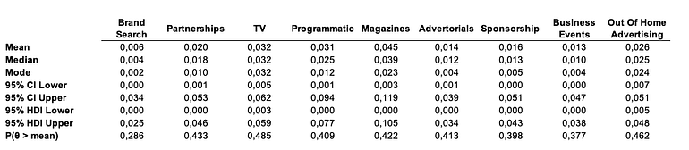
In Figure 12, we describe the mean, the median, the mode, the confidence interval (CI), the highest density interval (HDI) of posterior distributions, and the probability to find a value higher than the mean, P(θ > mean). We can see evidence of power-law behavior in most of the channels:

• Most channel influence distributions have significant right skewness across channels. The P(θ > mean) values cluster around 0.4 to 0.5, with the ‘Brand search’ channel having the lowest value (0.286).
• The ranges of HDI reveal a consistent asymmetry across different channels.
• CI upper/lower ratios maintain proportionality across influence levels, which could suggest that channels behave like systems with self-organized critically (SOC) dynamics, pointing to a phase transition between two regimes.
• Channels with high influence, like ‘TV ‘or ‘Magazines’ likewise present broader HDI ranges (0.003–0.119), which could imply a diversity of interconected influence mechanisms or sub-systems (HOT mechanism).
• Channels showing narrower HDI ranges (0.001–0.051), like ‘Programmatic’ and ‘OOH’ are more specialized channels with an important influence (0.031 and 0.026). These channels are very valuable for future investments, despite not being the most influencing nor the most stable. The reason is that these channels show simpler internal dynamics, which makes them more stable with time, so we can expect similar influence in varying contexts.

Analyzing long tails in channel influence distribution can be very useful to build a portfolio. We should allocate 40–50% to high-HOT channels, 30–40% to more stable channels, and 10–20% to emerging channels.

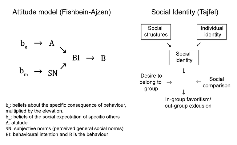
• 40–50%: High-influence channels like ‘TV’ or ‘Magazines’ also seem to follow a highly optimized tolerance mechanism (HOT). This suggests that within these channels, multiple complex mechanisms might interact to generate a global influence value, indicating that this channel could engage diverse audiences or involve various mechanisms of social influence and attitude change [21] in the overall channel impact.
• 30–40%: In an investment strategy, we should consider adopting channels with greater diversity to reduce uncertainty, even if they are not the most profitable. This approach not only reduces the risk of our investment across a wide range of uncertain scenarios, but it also proves to be highly valuable for new campaigns and reaching new audiences. Channels like ‘Programmatic’ and ‘OOH’ are more stable because they seem to involve fewer and less complex mechanisms.
• 10–20%: The remaining channels can be classified as emerging channels, offering opportunities in niche markets, such as accessing audiences not reached by other channels or supporting as the starting point of a viral campaign.

The emergence of power-law behavior and HOT mechanisms in our results is a true representation of the properties of marketing systems rather than a consequence of our prior distribution selection. The consistency of patterns across channels like asymmetric uncertainty, the proportionality in CI upper/lower ratios, the clustering of P(θ > mean) values around 0.4–0.5, and the evidence that different channels show different behaviors despite using the same prior distribution, support this interpretation.

Part 2: Response Curve Analysis

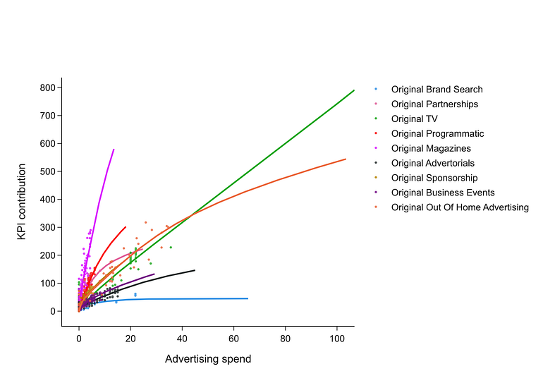
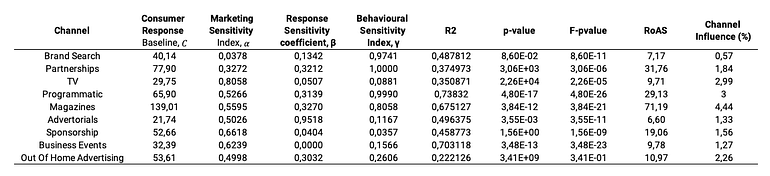
We are using Equation 2 to model the consumer response curves obtained from the Bayesian model. As we have seen, this model also follows a complex system point of view where we can find mechanisms like power law response, phase transitions and critical points, highly optimized tolerance mechanisms (HOT), and self-organized critically systems (SOC). The parameters obtained from fitting data with Equation 2 are shown in Figure 14.

• Marketing Sensitivity Index (α): High values in ‘TV’ and ‘Sponsorships‘ (0.80584 and 0.6618) indicate multiple interacting mechanisms aligned with HOT. These values correlate with the broad HDI ranges observed in influence distributions for these channels. As this index reflects the system's capacity for rapid scaling, channels with low values as ‘Brand Search’ (0.0378) suggest simpler, more focused mechanisms. It also aligns with narrower HDI ranges in influence distributions. Channels with low values provide more predictable but limited scaling potential.
• Response Sensitivity (β): ‘Advertorials’ and ‘Magazines’ (0.9518 and 0.3270) show rapid phase transitions that match observed critical points in influence distributions. It indicates the system's proximity to a HOT state, meaning that there are different complex mechanisms for the overall channel response. Channels with low values as ‘Business events’ and ‘Sponsorship’ (0.0000 and 0.0404) indicate more gradual transitions between states, equivalent to stable regions in influence distributions from Figure 11. Channels with low values indicate that the response range has not a clear saturation point.
• Behavioral Sensitivity Index (γ): High values in ‘Partnerships’ and ‘Brand Search’ (1.0000 and 0.9741) describe a strong percolation effect with large audience clusters. It maps to asymmetric tails in influence distributions in Figure 11 for these channels. These high values illustrate efficient advertising network diffusion. Channels with low values as ‘TV’ and ‘Sponsorship’ (0.0081 and 0.0357) show limited network effects, meaning we are reaching a more fragmented audience. This observation also corresponds to more symmetric influence distributions in Figure 11, describing different response mechanisms working together.

These coefficients have no direct relation with the metrics used for analyzing the channel influence distribution as they describe different processes. However, the underliying mechanisms are the same.

Executive Summary (or practical action plan)

• Channel performance structure

Marketing channels naturally develop long-tail distributions of influence. These patterns aren’t errors—they represent optimal system behavior. Different channels show distinct patterns that reveal their underlying mechanisms

• Channel types and behaviors

Power Players (e.g., TV, Magazines): Show complex, interconnected influence mechanisms (HOT mechanisms).

Specialists (e.g., Programmatic, OOH): Focused, stable performance (simple mechanisms).

Emerging Channels: Exhibit developing patterns with growth potential (reach new audiences).

• Network effects

Strong network effects appear in channels like Brand Search (γ = 0.9741). Some channels show fragmented audience response (TV, γ = 0.0081). Response patterns predict viral potential and audience clustering.

• Portfolio allocation strategy

40–50%: Invest in ‘Power Players’ (high Marketing Sensitivity Index and long tail influence distribution).

30–40%: Allocate to ‘Specialist’ channels for stability and risk mitigation.

10–20%: Set aside for emerging channels with growth potential.

• Risk management

Leverage channel diversity rather than focusing solely on top performers. Use channels with different audience clustering patterns—are we interested in new audiences? Do we want to focus on a unique audience to maximize the KPI? — . Check phase transitions in channel performance.

• Immediate actions

Analyze your channel portfolio for distribution patterns. Identify which channels are ‘Power Player’ vs. ‘Specialist’ (complex mechanisms vs. simpler ones). Begin reallocation based on the 50–30–20 framework.

• Monitoring framework

Check the Marketing Sensitivity Index (α) for scaling potential. Monitor the Behavioral Sensitivity Index (γ) for network effects—are we reaching multiple audinces? or is our audience acting as a homogeneous group?Control Response Sensitivity Index (β) for saturation signals.

• Optimization steps

Adjust spend when channels approach critical points. Balance investment across different mechanism types (more complex and simpler ones). Use network effect indicators to time campaign scaling.

Conclusions

Complex systems theory potential allows us to identify these mechanisms even in different processes. This is why complex systems approach, despite including the intimidating word ‘complex’, is overlay useful. If we look at the investment strategy coming from the channel distribution analysis, we can see that the conclusions we get using complex systems analysis tools with the response curve are very similar. In our first analysis (long tails in channel influence distributions), we have concluded investing 40–50% in high-influence channels like ‘TV’ or ‘Magazines’ because they evidenced a HOT mechanism. These channels behave like a system formed of various subsystems interacting together, which gives the system considerable robustness. The response curve of these channels (our second analysis) shows high marketing sensitivity index values (α), describing as well a HOT mechanism behind. Both channels also show a low behavioral sensitivity index value (γ) that describes as well a system formed by different subsystems reaching a wide variety of audiences where each of these audiences is reacting to advertising campaigns differently. In both analyses (channel influence distribution and response curve), the key is understanding that both are strongly influenced by the presence of a HOT mechanism.

If we want a mathematical formalism linking both analyses, we could say that there exists a statistically significant correlation between the P(θ > mean) and the marketing sensitivity index (α). The first metric quantifies the presence of long tails in the distribution curve of a channel’s influence, that is, the probability of rare occurrences and exceptions. The second metric, as we explained when introducing Equation 4, describes a Power Law mechanism. Therefore, it is consisting that these two parameters correlate with each other, despite describing two different processes. This is proof that the underlying mechanisms are the same.

References

[1] Ajzen, I., & Fishbein, M. (2000). Attitudes and the Attitude-Behavior Relation: Reasoned and Automatic Processes. European Review of Social Psychology, 11(1), 1–33.

[2] Alalwan, A. A. (2018). Investigating the impact of social media advertising features on customer purchase intention. International Journal of Information Management, 42, 65–77.

[3] Anderson, C. (2012). The long tail. Effective Business Model on the Internet—Moscow: Mann, Ivanov & Ferber.

[4] Andriani, P., & McKelvey, B. (2007). Beyond Gaussian averages: redirecting international business and management research toward extreme events and power laws. Journal of International Business Studies, 38, 1212–1230.

[5] Berger, J. O. (2013). Statistical decision theory and Bayesian analysis. Springer Science & Business Media.

[6] Bohner, G., & Dickel, N. (2010). Attitudes and Attitude Change. Annual Review of Psychology, 62(1), 391–417.

[7] Broido, A. D., & Clauset, A. (2019). Scale-free networks are rare. Nature communications, 10(1), 1017.

[8] Carlson, J. M., & Doyle, J. (2002). Complexity and robustness. Proceedings of the National Academy of Sciences, 99(suppl_1), 2538–2545.

[9] Castellano, C., Fortunato, S., & Loreto, V. (2009). Statistical physics of social dynamics. Reviews of Modern Physics, 81(2), 591–646.

[10] Chan, D., & Perry, M. (2017). Challenges And Opportunities In Media Mix Modeling. Google Inc. .

[11] Chen, H., Zhang, M., Han, L., & Lim, A. (2021). Hierarchical marketing mix models with sign constraints. Journal of Applied Statistics, 48(13–15), 2944–2960.

[12] Clauset, A., Shalizi, C. R., & Newman, M. E. (2009). Power-law distributions in empirical data. SIAM review, 51(4), 661–703.

[13] Cont, R. (2001). Empirical properties of asset returns: stylized facts and statistical issues. Quantitative finance, 1(2), 223.

[14] Dubé, J. P., Hitsch, G. J., & Manchanda, P. (2005). An empirical model of advertising dynamics. Quantitative Marketing and Economics, 3(2), 107–144.

[15] Feinberg, F. M. (2001). On continuous-time optimal advertising under S-shaped response. Management Science, 47(11), 1476–1487.

[16] Finkel, E. J., & Baumeister, R. F. (2010). Attitude change. In Advanced Social Psychology : The State of the Science (pp. 117–245). Oxford University Press.

[17] Gelman, A., Carlin, J. B., Stern, H. S., & Rubin, D. B. (1995). Bayesian data analysis. Chapman and Hall/CRC.

[18] Glattfelder, J. B. (2019). Information — consciousness — reality: how a new understanding of the universe can help answer age-old questions of existence. Springer Nature.

[19] Goldenberg, J., Libai, B., Solomon, S., Jan, N., & Stauffer, D. (2000). Marketing percolation. Physica A: statistical mechanics and its applications, 284(1–4), 335–347.

[20] Hill, A. V. (1910). The possible effects of the aggregation of the molecules of hemoglobin on its dissociation curves. J. Physiol., 40, iv–vii.

[21] Hunter, J. E., Danes, J. E., & Cohen, S. H. (1984). Mathematical models of attitude change. In Mathematical Models of Attitude Change (Vol. 1). Academic Press.

[22] Jensen, H. J. (1998). Self-organized criticality: emergent complex behavior in physical and biological systems (Vol. 10). Cambridge University Press.

[23] Jin, Y., Wang, Y., Sun, Y., Chan, D., & Koehler, J. (2017). Bayesian Methods for Media Mix Modeling with Carryover and Shape Effects.

[24] Johansson, J. K. (1979). Advertising and the S-curve: A new approach. Journal of Marketing Research, 16(3), 346–354.

[25] Liska, A. E. (1984). A Critical Examination of the Causal Structure of the Fishbein/Ajzen Attitude-Behavior Model. Social Psychology Quarterly, 47(1), 61.

[26] Marin, J. (2024). Social Dynamics of Consumer Response: A Unified Framework Integrating Statistical Physics and Marketing Dynamics. arXiv preprint arXiv:2404.02175.

[27] Marković, D., & Gros, C. (2014). Power laws and self-organized criticality in theory and nature. Physics Reports, 536(2), 41–74.

[28] Munoz, M. A. (2018). Colloquium: Criticality and dynamical scaling in living systems. Reviews of Modern Physics, 90(3), 031001.

[29] Neal, R. M. (2012). MCMC using Hamiltonian dynamics. arXiv preprint arXiv:1206.1901.

[30] Newman, M. E. J. (2005). “Power Laws, Pareto Distributions and Zipf’s Law.” Contemporary Physics, 46(5), 323–351.

[31] Prest, A. R. (1949). Some Experiments in Demand Analysis. The Review of Economics and Statistics, 31(1), 33.

[32] Simon, J. L., & Arndt, J. (1980). The shape of the advertising response function. Journal of Advertising Research.

[33] Sornette, D. (2006). Critical phenomena in natural sciences: chaos, fractals, self-organization, and disorder: concepts and tools. Springer Science & Business Media.

[34] Working, E. J. (1927). What Do Statistical “Demand Curves” Show? The Quarterly Journal of Economics, 41(2), 212–235.

Appendix I: Investment decision tree

Footnotes

¹ Other models, like the well-known Robyn from Meta, uses a Ridge regression to estimate the channel influence. Ridge regression provides a single point estimate for each channel with standard errors under normality assumptions. This approach assumes symmetric uncertainty and is based on asymptotic approximations, not being able to capture the natural skewness in channel effects due to exceptions and rare occurences.