Explainable Deep Neural Networks

Nature is an infinite sphere whose center is everywhere and whose circumference is nowhere.
B. Pascal

Introduction

For some years, black box machine learning has been criticized for its limits in extracting knowledge from data. Deep Neural Networks (DNNs) are one of the most well-known of the ‘black box’ algorithms. Deep Neural Networks (DNNs) are the most widely used and successful image classification and processing technique today. But when it comes to structured data (the most common data problem),, there is still a controversial about its advantage. Efforts have been made in recent years to produce explainable machine learning techniques, with the goal of providing a stronger descriptive approach to algorithms as well as additional information to users, hence enhancing data insights. In this work we propose a new way to make Deep Neural Networks more comprehensible when converting data encoded into practical knowledge. In each hidden layer representation, the data structure will be examined to gain a clear idea of how a deep neural network transforms data for classification purposes.

The puzzle of deep learning

The field of deep learning mathematical analysis (Berner, J. et al. 2021) is attempting to understand the mysterious inner workings of neural networks using mathematical methodologies. One of the key goals of this research is to understand what a neural network actually does as it processes data. Deep Neural Networks (DNNs) transform data at each layer, creating a new representation as output. In a classification problem, DNNs seek to divide the data into distinct categories, improving this process layer by layer until the final output is produced. Because natural data makes lower-dimensional manifolds in its embedding space, the manifold hypothesis says that this task can be thought of as separating lower-dimensional manifolds in a data space (Fefferman C., 2016; Olah C., 2014).

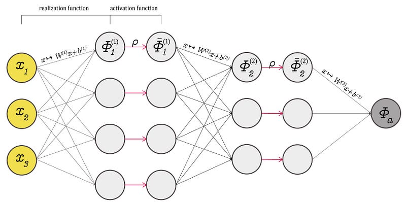
A realization function, (an affine transformation), and a component-wise activation function, are what connect DNN layers. Consider the fully connected feedforward neural network depicted in Figure 2. The network architecture can be described by defining the number of layers \(N\), \(L\), the number of neurons, and the activation function. The network parameters are the weights matrix W and the bias vectors b. Each layer’s output is a new way of describing inputs. This is why they are referred to as representations, as they are essentially abstractions over input data. For each layer, \(Φ(x , θ)= Wx+b\), with parameters \(θ = (W , b)\). The weights matrix is \(W\), while the bias vector is \(b\).

The activation function is crucial in determining how neural networks are connected and which information is transmitted from one layer to the next. Finally, it controls information exchange, allowing neural networks to “learn” from data. What they learn and why they learn it remains a difficult topic. Some researchers even argue that DNN can learn something particular about the data and that this research is shared by several layers. So the argument that a layer learns something and then passes a representation to the next layer, which learns something else, is partially correct.

Topology of data

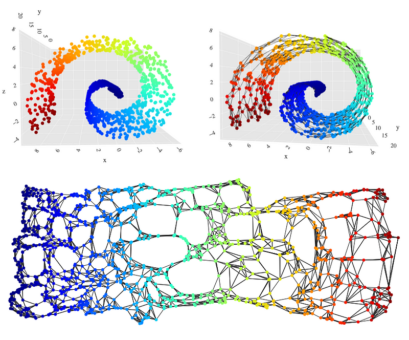
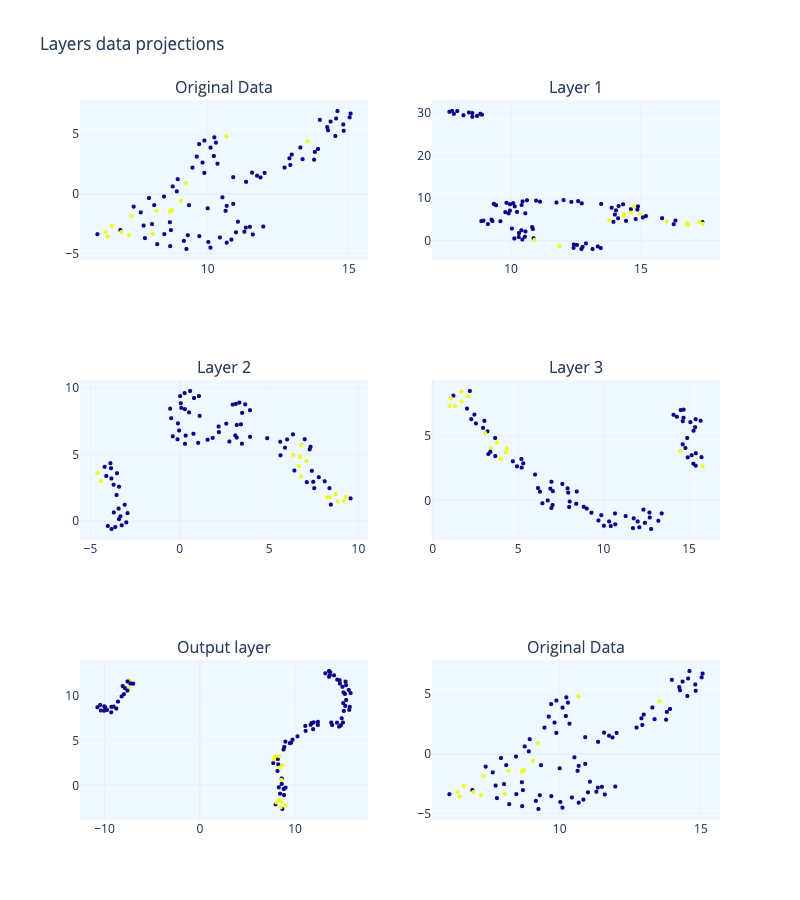
Visualizing high-dimensional data representations via dimensionality reduction is a well-known technique for examining deep learning models. In Figure 3, we can see the layer representation for a network with an architecture, \(a= ((33, 500, 250, 50, 1), ρ)\).

Aside from dimensionality reduction, there are alternative techniques for visualizing high-dimensional models. Topology analyzes the connection information of elements in a space and deals with qualitative geometric information. Topological data analysis (TDA) uses category theory, algebraic topology, and other pure mathematics methods to enable a practical investigation of data form (Carlsson G., 2009). High-dimensional data sets significantly limit our ability to visualize them. This is why TDA can help us improve our ability to visualize and analyze information. The most frequently observed data topologies include connected components, loops, voids, and so on.

The curse of dimensionality is a major challenge when analyzing high-dimensional data representations in deep neural networks. In high-dimensional space, points are widely dispersed, and when a DNN transfers data from one layer to another with a different number of dimensions, the Euclidean distances between points and the distance of a point to a subset tend to increase. Topology is a branch of mathematics that studies the properties of geometric objects that are independent of the chosen coordinates, meaning that these properties do not change even if the object is stretched, bent, or otherwise deformed. This makes topology particularly useful for analyzing deep neural network representations, as it allows for the analysis of the underlying structure of the data without being affected by the scale or orientation of the data points.

Topology avoids the quantitative values of the distance functions and replaces them with the notion of “infinite nearness” of a point to a subset in the underlying space (Carlsson G., 2009).

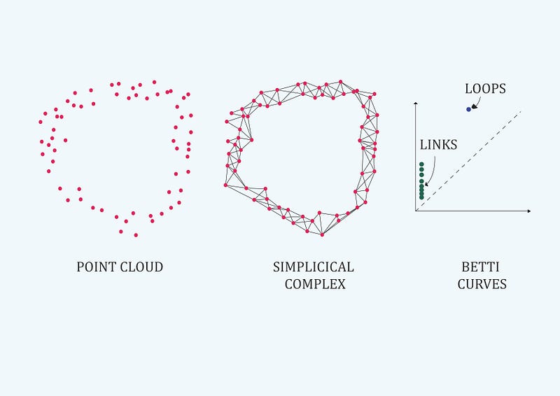
Topology data analysis methods follows a basic routine: we come across a topological space (a representation of a high dimensional dataset ) and we need to find its fundamental group (data relations as links, loops or voids). But our data set is an unfamiliar space and it’s too difficult to look at explicit loops and relations. Then we look for another space that is homotopy equivalent to ours (Carlsson G., 2009), and whose fundamental group is much easier to compute. Since both spaces are homotopy equivalent, we know fundamental group in our space is isomorphic to fundamental group in the new space (gives the same data connectivity information). And its a coordinates-free process . Level-one connectivity information is related to data links, level-two connectivity information to data loops and level-three to voids (figure 4 shows level-one in green color and level-two in blue color.

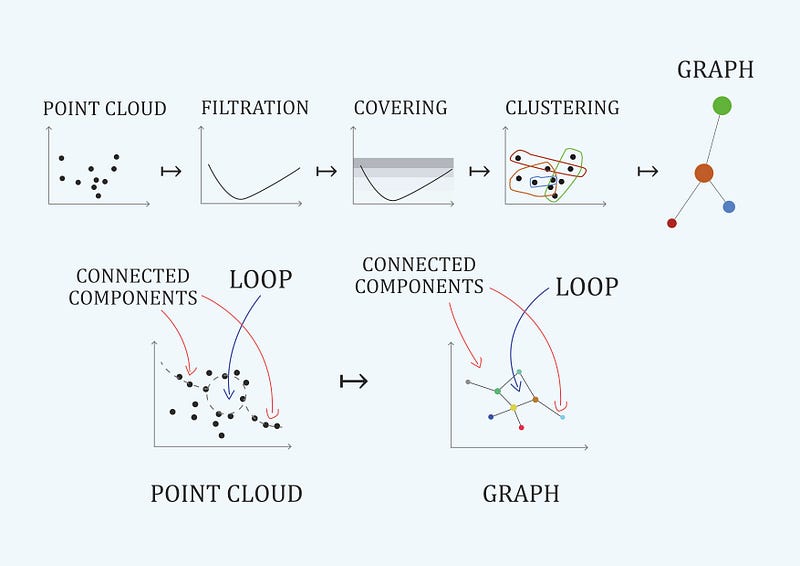
Topological data analysis provides both quantitive methods and tools for qualitative understanding of high-dimensionality data through direct visualization. An example is the mapper algorithm represented in Figure 5 (Carlsson G., 2009). Quantitative data analysis will find the fundamental group of representation, and qualitative data analysis will bring other qualitative insights about data.

Topological signatures of a space are its fundamental groups. In TDA these signatures are the quantitative elements used to characterize the data space.

To intuitively understand what is Data Topology, we invite you to read this wonderful post: The Mathematical Shape of Things to Come from Tang Yau Hoong, published in Quanta Magazine.

As corollary we can say that Topological Data Analysis is about finding connections

Understanding the topology of deep nets representations: a real example

In this post, we propose that using Topological Data Analysis on the representations of deep neural networks (DNNs) can help us better understand how these networks function and what information can be gleaned from each layer. To demonstrate this, we will use a dataset provided by the Government of India as part of a Drug Discovery Hackathon, which is also available on Kaggle. The dataset includes a list of drugs that have been tested for their effectiveness against Sars-CoV-2, along with additional chemical details for each molecule obtained from the PubChem library. The final dataset includes 100 tested molecules, each with 40 features, including the pIC50 value, which is the negative logarithm of the half maximal inhibitory concentration and is used as a measure of a substance’s efficacy as an inhibitor. The goal of this analysis is to develop a classification method for these molecules based on their effectiveness against Sars-CoV-2. The dataset also includes six blinded molecules, which do not have the pIC50 value and can be used for predictive tasks.

We used the Giotto-tda library to perform TDA computations. Library gtda is a high-performance topological machine learning toolbox written in Python. The real advantage of using gtda, in my opinion, is its direct integration with scikit-learn and support for tabular data, time series, graphs, or pictures. Both assets make it simple to construct machine learning pipelines. For Deep Neural Networks we are using Keras library.

Deep neural network architecture

In our experiment we have used a fully connected neural network with architecture, \(a = ((33, 500, 250, 50, 1), ρ)\). It is a basic graph with three hidden layers. We have built the network with Keras functional API in order to make the different experiments more reproducible. The functional API can handle models with non-linear topology.

# 'clean' is the pandas data frame with the data, 
# and 'pIC50' is the label feature.

input_dim = len(clean.drop(columns='pIC50').columns) 
model = Sequential()

#The Dense function in Keras constructs a fully connected neural network layer, automatically initializing the weights as biases.

#First hidden layer
model.add(Dense(
               50, 
               activation='relu',
               kernel_initializer='random_normal,
               kernel_regularizer=regularizers.l2(0.05),
               input_dim=input_dim)
)

#Second hidden layer
model.add(Dense(40, activation='relu',  
          kernel_initializer='random_normal',
          kernel_regularizer=regularizers.l2(0.05) ))
#Third hidden layer
model.add(Dense(20, activation='relu',  
          kernel_initializer='random_normal',
          kernel_regularizer=regularizers.l2(0.05) ))#Output layer
model.add(Dense(1, activation='sigmoid',  
          kernel_initializer='random_normal',
          kernel_regularizer=regularizers.l2(0.05) ))
          
model.compile(optimizer='adam',   
             loss='binary_crossentropy',
             metrics=['accuracy'])

As mentioned earlier, activation functions are critical in mapping data from one layer to another. There are two kinds of activation functions that we’re interested in: invertible (continuous functions with continuous inverses) and not invertible. tanh , sigmoid or softplus, are examples of first-class functions, and ReLU is an example of a non-invertible function. Activation functions can be invertible, but a neural network as a whole, even with invertible activation functions, is not invertible in general.

At this point, it’s worth recapping. We want to look into representation’s topology in a deep neural net. The key question will therefore be whether topological signatures preserve from one representation to the next. The answer can be found in category theory: a construction that converts objects (for example, de DNN representations) from one category to objects from another is functorial if:

• it can be extended to a mapping on morphisms, and
• while preserving composites and identity morphisms (Riehl E., 2017).

Such constructions define morphisms between categories, called functors. Such functors or constructions define morphisms between categories as \(F : C → D\) between categories \(C\) and \(D\) . As a result, the task is limited to determining if data mapping from one layer to another is a functor. A functor describes an equivalence of categories so the objects in one category can be translated into and reconstructed from the objects of another category.

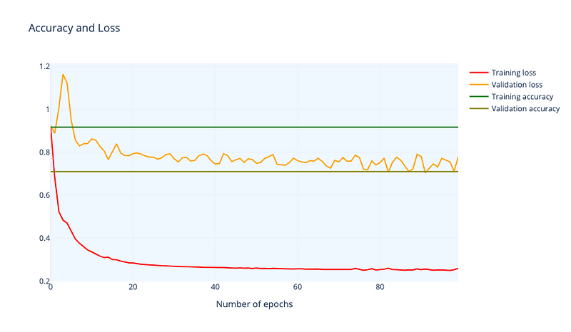
To check functionality in a DNN first, we analyze the accuracy and loss of our DNN architecture (Figure 6).

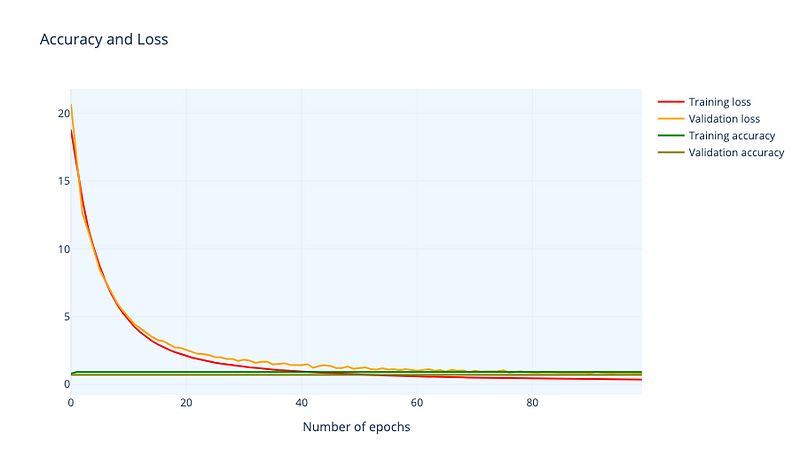
Training accuracy is 0.916 and training accuracy is 0.709. Remember we have a small dataset so accuracy is affected. Now we calculate the topological signatures of every representation(it is, finding fundamental groups in for each layer representation). We do this with gtda library, using Vietori-Rips filtration (Carlsson G., 2009). Results can be seen in Figure 7.

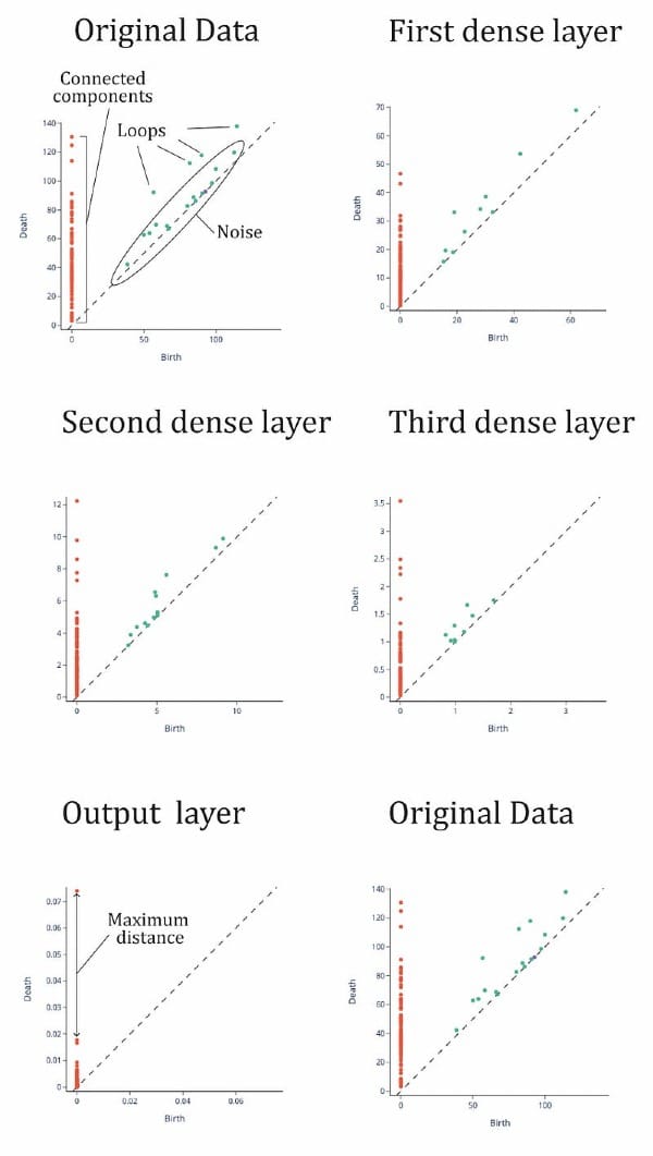
To understand this figure, we can consider the following: the orange points represent data points that are “close” together in the topological space, while the green points represent “loops” or clusters of points. The green points close to the diagonal may be considered noise, or incompletely formed loops. The orange points also indicate the size of the set and can be used as a quantitative way to characterize the space, known as topological signatures. In Figure 7, we can see that the topological signatures from the input layer to the third hidden layer are maintained, with four distinct loops and several connected points. There is also an orange point on the vertical line that is separated from the others. In a binary classification task, we would expect to see two distinct clusters of points on the vertical line representing the two categories, otherwise the set may not be classifiable.

This is clear in the output layer where we can see a point remarkably away from the rest of points, meaning that there are two categories and that one of them is much smaller than the other (one has only one point and the other one has more than 10 points). Then DNN has separated the connected points until she got a clear separation, a maximum “distance” or minimum “nearness” between points. It has binary classified the dataset¡ So, the topological signatures seems to be the same but in the output function where we have asked the DNN to manipulate this to make a classification. So the transformation between representations is functorial: composites and identity morphisms are preserved.

We have repeated the experiment varying several hyper-parameters. The most interesting conclusion is that functoriality seems more dependent on network width that on activation function invertibility.

We have experimented with a network architecture \(a = ((33, 50, 25, 10, 1), ρ)\). Accuracy and Loss are very similar to the wider architecture (Figure 8). Then we performed the same Vietory-Rips filtration (Figure 9). We see that topological signatures are quite different from the original data set. In the first hidden layer, we see less loops that completely disappear in the second hidden layer (we found basically noise). From the second layer, topological signatures are not mapped.

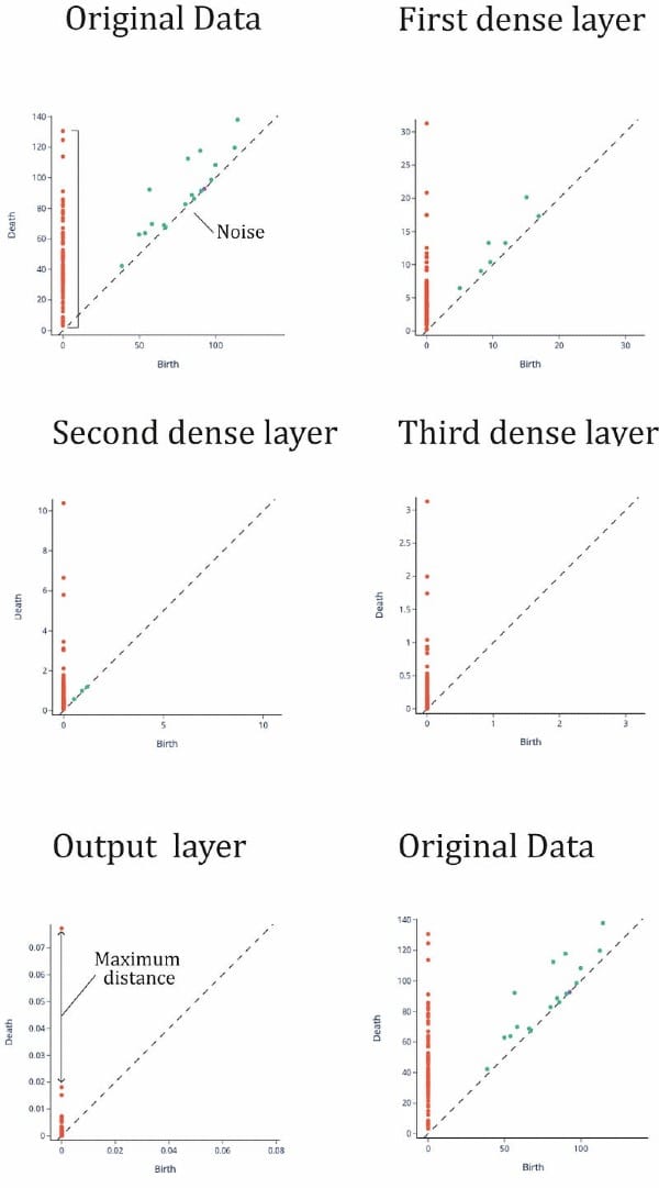
The neural network is able to separate the connected points even with a wider architecture, which may seem counterintuitive because it suggests that DNN does not need to take topological signatures into account in order to perform accurate separation. However, it is possible to achieve this through relatively simple operations. DNN “manipulates” the topology of the data by altering the “closeness” between points in such a way that identity morphisms are not preserved.

Another different topic is that it should be necessary to consider the equivalence of categories during the learning process. When we consider small datasets, despite we are getting relative high accuracy levels, we should try to do it better. Topological data analysis gives us tools to double test network performance in the learning process.

Qualitative information

We have seen a quantitative topological approach. But topology offers qualitative understanding tools that can be very interesting. Mapper algorithm introduced in Figure 5 is a very interesting ‘visualization’ algorithm that can enhance the performance of dimensionality reduction algorithms. Mapper algorithm can be naturally seen as a clustering algorithm with a conversion to a graph with directed edges. In figure 10 we can see the results of applying mapper algorithm to layer’s representation in the network with architecture \(a = ((33, 500, 250, 50, 1), ρ)\) -wide layer. The nodes are colored with a scale of ‘pIC50' values (our label feature). Despite we have been performing binary classification ( 0 for negative pIC50 values and 1 for positive), we are interested now in a regression point of view to get beer insights. We have implemented mapper algorithm with gtda library. Mapper’s difficulty in choosing hyperparameters filter, cover and cluster data.

""" 1. Define filter function – can be any scikit-learn transformer. It is returning a selection of columns of the data """

filter_func = Eccentricity(metric= 'euclidean') 

"""2. Define cover"""

cover = CubicalCover(n_intervals=20, overlap_frac=0.5)

""" 3. Choose clustering algorithm – default is DBSCAN""" 

clusterer = DBSCAN(eps=8,
                   min_samples=2,
                   metric='euclidean')
                   
""" 4. Initialise pipeline """

pipe_mapper = make_mapper_pipeline(filter_func=filter_func,
                                   cover=cover,
                                   clusterer=clusterer, 
                                   verbose=False,
                                   n_jobs=-1)
                                   
""" 5. Plot mapper """

plotly_params = {"node_trace": {"marker_colorscale": "RdBu"}}fig = plot_static_mapper_graph(
       pipe_mapper,
       X,
       layout='fruchterman_reingold',
       color_variable =clean['pIC50'],
       node_scale = 20,   
       plotly_params=plotly_params
)
fig.show(config={'scrollZoom': True})

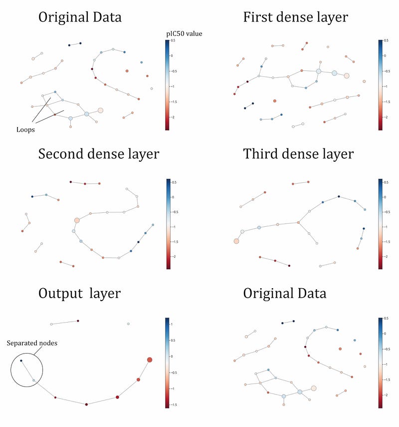
We see in figure 10 the mapper algorithm applied for input, hidden and output layers. Mapper in the input layer shows some “loops”, several connected component of different length, and some not-connected components (isolated nodes). We can also see loops in hidden layer 1, but not in the following layers. In the input layer we see blue points (positive value of pIC50) and red points (negative values of pIC50) totally mixed. With this graph plot, we can’t imagine an easy way to separate blue points from red points. But output layer shows what deep neural network have worked this separation: nodes with blue color and red color are very easy to divide because blue color are in the end of the connected component. We could easily cut the connection and we will have a binary classification. We can see we needed three hidden layer to perform this separation. If we look at the third layer, this separation is still not possible so another transformation have been necessary (output layer).

DNN approaches the classification problem by attempting to "connect" as many data points as possible in the mapper representation. The output layer generally consists of a main connected branch, as well as an isolated node and a two-node connected component. The points in this layer tend to be more connected compared to earlier layers in the network.

Another interesting feature from mapper algorithm is that you can visualize every node, extract the data points and translate insights directly from the original data set (Figure 11). We see mapper algorithm with the nodes translated to data points, specifically to a feature that is related to molecule drawing. Last but not least we can visualize the graph for every feature in the input data set and for every neuron inside the hidden layers.

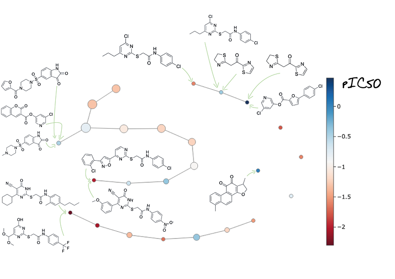
This feature from mapper can be useful for example to monitor how each molecule is placed in the graph in every layer.

Conclusions

In this research, we have examined the use of neural networks for image classification and structured data classification. While there have been some studies on the use of neural networks for image classification, there are fewer examples of their use for structured data classification. We have demonstrated the potential for using Topology Data Analysis as a tool for understanding the processes used by DNNs in completing tasks, and for improving their performance. Additionally, we have found that DNNs can achieve similar levels of accuracy whether or not data identities are preserved, though this has only been tested on small datasets. It may be worth exploring the use of preserving topological signatures as a metric for evaluating DNN accuracy when learning from data.

References

• Berner, J., Grohs, P., Kutyniok, G., & Petersen, P. (2021). The Modern Mathematics of Deep Learning. ArXiv, abs/2105.04026.
• C. Olah (2014). Neural Networks, Manifolds, and Topology. C. Olah blog.
• C. Fefferman, S. Mitter, & H. Narayanan (2016).Testing the manifold hypothesis. Journal of the Amer. Math. Soc. 29, 4, 983–1049.
• G. Carlsson. (2009) Topology and data. Bull. Amer. Math. Soc. 46 , 255–308.
• E. Riehl. (2017) Category theory in context. Courier Dover Publications.

You can find the code used in this article here.