From Newton to Gen AI

Introduction

Multiple facts are needed to answer a multi-hop question-answering (QA), which is essential for complex reasoning and explanations in Large Language Models (LLMs). QA quantifies and objectively tests intelligent system reasoning. Due to their unambiguous correct solutions, QA tasks reduce subjectivity and human bias in evaluation. QA functions can evaluate deductive reasoning, inductive reasoning, and abductive reasoning, which involves formulating the most plausible answer from partial knowledge.

We face several challenges in improving the model’s reasoning processes. One of the most important demands is model interpretability and explainability. Large AI models, especially deep neural networks, are hard to understand, which makes it hard to evaluate them accurately and come up with human-friendly explanations for their decisions and conclusions. Another important goal for improving the reasoning process is to ensure that reasoning processes are robust to minor variations in input or context, as well as to develop models that can generalize reasoning skills across different domains and types of questions.

The Power of Physical Analogies in AI

Physics’ significant excellence in formulating complex phenomena using advanced mathematical frameworks suggests that comparable approaches could be used effectively in other domains, such as artificial intelligence and cognitive research. The results of physics-based approaches in a number of scientific domains provide compelling evidence for exploring their applicability in AI, particularly in the context of assessing and improving models’ reasoning capacities. Similar to how physicists use mathematical models to explain the behavior of fundamental particles, quantum fields, and particle states, we propose using analogous formalisms to describe the dynamics of reasoning in a model's embedding space.

Introduction to Hamiltonian mechanics as a new frontier

The Hamiltonian formalism provides an effective mathematical framework for developing conservative mechanical system theory and is a geometric language for multiple fields of physics. Imagine yourself on a playground swing. When you swing, you move back and forth, up and down. A Hamiltonian system is a special way of representing the swinging motion. If someone is watching you, she may observe two things: where you are (position) and how quickly you are moving (speed). There’s a specific rule that explains how these two items change over time. Unless somebody outside pulls you, the swing’s overall energy (how high you go and how fast you move) remains constant (conservation).

The Hamiltonian formalism provides an effective mathematical framework for developing conservative mechanical system theory and is a geometric language for multiple fields of physics. A Hamiltonian can be defined with the following 2n ordinary differential equations:

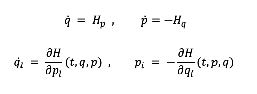
where 𝐻 = 𝐻(𝑡,𝑞,𝑝) is the Hamiltonian, 𝑞 and 𝑝 are the position and momentum vectors of a mechanical system with 𝑛 degrees of freedom, and 𝑡 is the time. For the purpose of this experiment, we can define the Hamiltonian, 𝐻, of a system as:

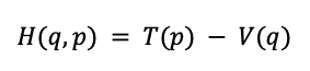
where position and momentum vectors of a mechanical system with 𝑛 degrees of freedom, 𝑇(𝑝) is the kinetic energy, and 𝑉(𝑞) is the potential energy of the system. Each point in phase space represents a unique state of the system, defined by its position and momentum coordinates (𝑞, 𝑝).

Symplectic Geometry: The Hidden Structure of Dynamical Systems

Symplectic geometry is a branch of differential geometry that uses mathematical frameworks to describe the evolution of classical mechanical systems. It is especially useful for studying energy-conserving systems such as planetary motion or pendulum oscillations. Imagine you’re solving a special puzzle. This puzzle has two elements that always fit together: where something is (for example, where a toy vehicle is on a track) and how fast it’s moving. Symplectic geometry is a set of rules for this puzzle that explain why these two pieces are always connected in a unique way. When you move one piece, the other must change in a specific pattern. No matter how you twist and bend the problem, these rules always apply. The amazing thing is that these rules allow us to predict how things will move in the future, even if the system is very complex.

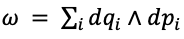
Symplectic geometry is the study of symplectic manifolds, which are smooth manifolds with even dimensions and a closed, non-degenerate differential 2-form known as the symplectic form. This form represents the fundamental structure of phase space in Hamiltonian mechanics. In local coordinates (pi, qi), a standard symplectic form can be written as

According to Liouville’s theorem, these structures preserve phase space volume and also ensure the conservation of certain geometric properties under the flow of Hamiltonian vector fields. The Forest-Ruth algorithm is a specific type of symplectic integrator. Symplectic integrators are schemas to do numerical integration that preserve the symplectic structure of Hamiltonian systems. This is very important for keeping basic properties like energy conservation over long periods of time. Formally, the Forest-Ruth algorithm is a 4th order symplectic integrator. A symmetric nth order symplectic algorithm advances this system temporally with Hamiltonian

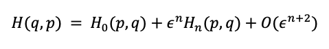
In essence, this algorithm adds two error terms to the Hamiltonian: the first one reflects the numerical method's error term, and the second one reflects higher-order errors.

From Physical Systems to AI Reasoning

In our model reasoning context, the Hamiltonian system can be analogous to the following quantities:

• 𝑞 represents the current state of reasoning
• 𝑝 represents the change in reasoning
• 𝑇(𝑝) — kinetical energy — represents the “cost” of changing the reasoning state
• 𝑉(𝑞) — potential energy — represents the “relevance” of the current reasoning state

The reasoning phase space (p,q) inherits the symplectic structure discussed earlier. This implies that our reasoning Hamiltonian will preserve certain geometric properties as it evolves, analogous to the conservation of phase space volume in dynamical systems.

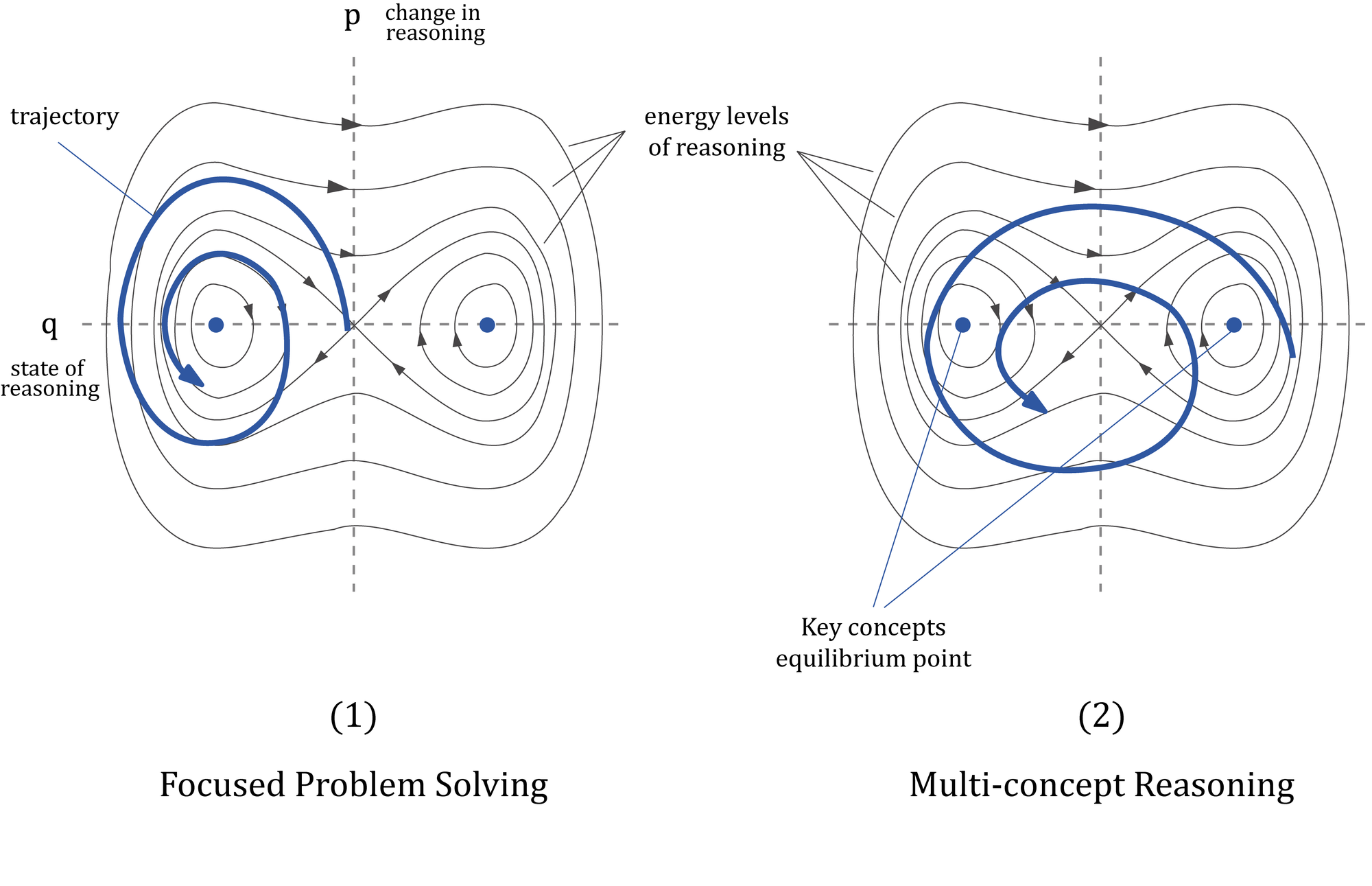
Figure 1 shows how Hamiltonian dynamics can guide our model optimization. Figure 1 illustrates a phase plot for a reasoning system, with the q-axis representing the current state of reasoning, similar to position in mechanical systems, and the p-axis representing the change in reasoning, equivalent to momentum. The contour lines represent the energy levels connected with reasoning. The blue lines represent potential reasoning paths and the evolution of reasoning over time in the phase space. Blue dots represent stable states or essential concepts. Figure 1.1 shows a focused problem-solving strategy characterized by tighter orbits around a single concept, indicating a strong attention on that concept. Figure 1.2 represents a multi-concept reasoning framework, with a bigger orbit containing many significant concepts, indicating the integration of various reasoning levels.

Implementing Hamiltonian-Inspired AI: The Code Explained

We performed our research using the OpenBookQA (OBQA) dataset, which provides a standard for assessing AI systems’ question-answering and reasoning abilities. Mihaylov et al. (2018) presented the OBQA dataset as part of their research on open-book question answering. It was designed to assess AI systems’ ability to reply to inquiries that require the integration of data from a specific text corpus with general knowledge.

1. Custom dataset

# Custom Dataset 
class OBQADataset(Dataset): 
    def __init__(self, texts, labels, tokenizer, max_length): 
        self.inputs = tokenizer( 
            texts,  
            padding=True,  
            truncation=True,  
            max_length=max_length,  
            return_tensors="pt" 
            ) 
        self.labels = torch.tensor(labels, dtype=torch.long) 
 
    def __len__(self): 
        return len(self.labels) 
 
    def __getitem__(self, idx): 
        return {key: val[idx] for key, val in self.inputs.items()}, self.labels[idx]

We developed a custom dataset class, like OBQA, for several reasons. This class contains the data preparation logic, making it simpler to manage and reuse. By deriving from torch.utils.data.Dataset, the dataset becomes compatible with PyTorch’s DataLoader, allowing for efficient batch processing and loading during training. It also manages the text data tokenization process, transforming raw text into a format that can be fed into a neural network while ensuring that all data samples are treated consistently, including padding and truncation to a defined maximum length. The getitem method enables lazy data loading, which saves memory by loading only the necessary samples when they are needed.
This module enables easy customisation of data preprocessing stages particular to the OBQA (OpenBookQA), such as translating labels to the proper tensor format for training. The len method is a simple approach to determining the total number of samples in the collection. Finally, it allows for the generation of batches with multiple input tensors (such as input_ids, attention_mask, and so on) and their related labels.

2. Custom optimizer

We have developed a custom optimizer named “Advanced Symplectic Optimizer”. This approach is consistent with the Hamiltonian dynamics framework that we are going to use to optimize AI reasoning. This optimizer uses a symplectic integrator (Forest-Ruth method) that is intended to preserve the geometric structure of Hamiltonians. Symplectic integrators are known for their long-term stability in simulating conservative systems, which may result in more stable and consistent training. By keeping to the Hamiltonian structure, it seeks to conserve the system’s “energy” during optimization, potentially leading to improved convergence properties. It uses an adaptable step size dependent on the system’s current state, allowing for more accurate updates. This optimizer also uses a momentum-based strategy, which can aid in navigating tight valleys in the loss landscape more successfully.

How does it work? It sets initial parameters including learning rate (lr), momentum decay (beta), and a small epsilon to ensure numerical stability.
The momentum is then updated by combining the prior momentum with the current gradient. It computes a Hamiltonian-like quantity by combining kinetic (based on momentum) and potential (based on gradient) energy terms. The step size is determined adaptively based on the current Hamiltonian value, which may allow for greater steps in flat sections and smaller steps in steep regions. The parameters are adjusted based on the calculated momentum and adaptive step size.

The Forest-Ruth algorithm, a fourth-order symplectic integrator, is approximated during the momentum and parameter update steps.
The adaptive step size computation

step_size = lr / (hamiltonian.sqrt() + eps)

modifies the effective learning rate to reflect the system’s current state. Momentum (state[‘momentum’]) can help speed up convergence and overcome local minima.

# Custom Optimizer 
class AdvancedSymplecticOptimizer(Optimizer): 
    def __init__(self, params, lr=1e-3, beta=0.9, epsilon=1e-8): 
        defaults = dict(lr=lr, beta=beta, epsilon=epsilon) 
        super(AdvancedSymplecticOptimizer, self).__init__(params, defaults) 
 
    @torch.no_grad() 
    def step(self, closure=None): 
        loss = None 
        if closure is not None: 
            with torch.enable_grad(): 
                loss = closure() 
 
        for group in self.param_groups: 
            for p in group['params']: 
                if p.grad is None: 
                    continue 
                grad = p.grad 
                state = self.state[p] 
 
                if len(state) == 0: 
                    state['step'] = 0 
                    state['momentum'] = torch.zeros_like(p.data) 
 
                momentum = state['momentum'] 
                lr, beta, eps = group['lr'], group['beta'], group['epsilon'] 
 
                state['step'] += 1 
 
                # Implement 4th order symplectic integrator (Forest-Ruth algorithm) 
                momentum.mul_(beta).add_(grad, alpha=1 - beta) 
 
                # Compute adaptive step size 
                kinetic = 0.5 * (momentum ** 2).sum() 
                potential = 0.5 * (grad ** 2).sum() 
                hamiltonian = kinetic + potential 
                step_size = lr / (hamiltonian.sqrt() + eps) 
 
                p.add_(momentum, alpha=-step_size) 
 
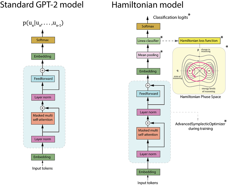
        return loss

3. Modified GPT-2 Model

The HamiltonianGPT2 class is a customized version of the regular GPT2LMHeadModel that has several unique features. The model adds a linear classification layer (self.classifier) on top of the GPT-2 architecture. This layer transfers the GPT-2 embedding dimension (config.n_embd) to two output classes, allowing binary classification. The forward method is overridden to include the classification task. It initially calls the parent class’s forward method to obtain the GPT-2 outputs. It requires only the hidden states (output_hidden_states=True). The model uses the last hidden state from GPT-2’s output. It performs mean pooling on the sequence dimension (pooled_output = hidden_states.mean(dim=1)). This generates a fixed-sized representation of the input sequence. The pooled output is passed on via the classification layer, which produces logits for binary classification.When labels are provided, the loss is calculated using CrossEntropyLoss. This enables the model to be trained on the classification task. The model provides both the classification logits and the loss. This makes it appropriate for training and inference.
The primary difference here is modifying the GPT-2 model, which was originally designed for language modeling, for use in binary classification. It achieves this by using GPT-2’s extensive representations and incorporating a task-specific categorization head. This method allows the model to leverage GPT-2’s pre-trained information while being fine-tuned for a given classification task.

class HamiltonianGPT2(GPT2LMHeadModel): 
    def __init__(self, config): 
        super().__init__(config) 
        self.classifier = nn.Linear(config.n_embd, 2)  # Binary classification 
 
    def forward(self, input_ids, attention_mask=None, labels=None): 
        outputs = super().forward( 
            input_ids,  
            attention_mask=attention_mask,  
            output_hidden_states=True 
            ) 
        hidden_states = outputs.hidden_states[-1]  # Get the last hidden state 
        pooled_output = hidden_states.mean(dim=1) 
        logits = self.classifier(pooled_output) 
 
        loss = None 
        if labels is not None: 
            loss_fct = nn.CrossEntropyLoss() 
            loss = loss_fct(logits, labels) 
 
        return (logits, loss)

4. Hamiltonian loss

We have developed an innovative method that combines ideas from Hamiltonian mechanics with classic classification loss, to develop a custom Hamiltonian loss function. This loss function is designed in this way for several reasons: To begin, the function compares the actual labels with the model’s predictions (logits) and determines the standard classification loss (cross-entropy loss). As a result, you know the model is picking up accurate input classifications. The sum of the L2 norms of all model parameters is computed by the added term param_norm.This could be seen as a way to quantify the “energy” or complexity of the model. A small penalty according to the model’s parameter norms is added by the reg_term (0.01 * param_norm). This pushes the model toward limited parameters, which is equivalent to keeping the “energy” low from a Hamiltonian perspective. Then we add the regularization term to the base loss to get the total loss.

This method is important because it encourages the model to discover solutions with low “energy” consumption by penalizing high parameter values. By limiting the model’s dependence on any one parameter, the regularization term helps mitigate the risk of overfitting. By keeping parameter values small, we can achieve stable gradients during training, which might improve convergence. For better understanding of the model’s interpretability-related behavior, the regularization term allows us to measure and control the model’s complexity.

def hamiltonian_loss(outputs, labels, model): 
    logits, base_loss = outputs 
    if base_loss is None: 
        loss_fct = nn.CrossEntropyLoss() 
        base_loss = loss_fct(logits, labels) 
    # Add regularization based on Hamiltonian principles 
    param_norm = sum(p.norm().item() for p in model.parameters()) 
    reg_term = 0.01 * param_norm  # Adjust coefficient as needed 
    return base_loss + reg_term

5. Fine-tuning GPT2 with our Hamiltonian approach

We are using a custom HamiltonianGPT2 model, which includes modifications to the regular GPT-2 design influenced by Hamiltonian approach. Based on this approach, our custom optimizer implements an adaptable step size and a symplectic integrator (Forest-Ruth algorithm). The training loop combines the standard loss and a regularization factor from Hamiltonian mechanics to form the hamiltonian_loss function.
The output_hidden_states=True setting in GPT2Config setup is used to analyze the internal representations of the model from a Hamiltonian approach. The application of K-fold cross-validation provides a rigorous method for assessing the generalizability and stability of our model. The evaluation offers a thorough analysis of the model’s performance and includes accuracy, precision, recall, and F1 scores. The use of DataLoader with custom samplers aligns with the need for efficient data processing in Hamiltonian-inspired optimization. We selected a small learning rate (5e-5) to complement the Hamiltonian-inspired optimization approach.
With this code structure, we carefully added the Hamiltonian approach to the GPT-2 model's process for fine-tuning the OBQA classification. It combines our new physics-inspired method with common deep learning techniques, which could result in more consistent, effective, and comprehensible AI reasoning optimization.

def evaluate_model(model, dataloader, device): 
    model.eval() 
    all_preds = [] 
    all_labels = [] 
 
    with torch.no_grad(): 
        for batch in tqdm(dataloader, desc="Evaluating"): 
            inputs = {k: v.to(device) for k, v in batch[0].items()} 
            labels = batch[1].to(device) 
 
            if isinstance(model, HamiltonianGPT2): 
                outputs = model(**inputs) 
                logits = outputs[0] 
            else: 
                outputs = model(**inputs) 
                logits = outputs.logits.mean(dim=1)  # Average over sequence length 
 
            preds = torch.argmax(logits, dim=-1) 
            all_preds.extend(preds.cpu().numpy()) 
            all_labels.extend(labels.cpu().numpy()) 
 
    accuracy = accuracy_score(all_labels, all_preds) 
    precision, recall, f1, _ = precision_recall_fscore_support( 
        all_labels,  
        all_preds,  
        average='weighted',  
        zero_division=0 
        ) 
 
    return accuracy, precision, recall, f1

Results and Implications

We have used both models, standard GPT2 and HamiltonianGPT2 in order to classify valid and invalid chains in the OBQA dataset. The dataset contains 998 records with Fact 1, Fact 2, question, answer, and a binary column indicating if the answer is correct or not. The results obtained using the standard GPT2 model have been the following:

#Evaluating Standard GPT-2 
 
Accuracy: 0.0200 
Precision: 0.010 
Recall: 0.0200,  
F1: 0.0138

An for our HamiltonianGPT2:

#Evaluating Hamiltonian GPT2 
 
- Without K-fold 
Accuracy: 0.8950 
Precision: 0.801 
Recall: 0.8950 
F1: 0.8454 
 
- With K-fold cross-validation 
Mean Accuracy: 0.9060 (+/- 0.0232) 
Mean F1 Score: 0.8627 (+/- 0.0338)

The fine-tuned model shows a dramatic improvement over the standard GPT-2 model, with accuracy increasing from 2% to 89.50%. The final test results are very close to the cross-validation results, which is a good sign. This suggests that the model is generalizing well to unseen data. The accuracy and recall are identical (0.8950), indicating that the model is performing consistently across classes. The slightly lower precision (0.8010) suggests a small tendency towards false positives.

The standard deviations in the cross-validation results are relatively small (2.32% for accuracy and 3.38% for F1 score), indicating consistent performance across different subsets of the data. Robustness: The cross-validation results being close to the final test results suggests that the model’s performance is robust and not just a lucky split of the data.

The fine-tuning process has been highly effective in adapting the model to your specific task. The consistent performance across cross-validation folds and the final test set suggests that the model generalizes well. The large improvement from the base model to the fine-tuned model suggests that your task requires specific adaptation that the base GPT-2 model couldn’t handle without fine-tuning. The high performance metrics suggest that your Hamiltonian-inspired approach is indeed adequate for this valid/invalid chain classification.

Broader implications

While benchmarking our model to standard GPT-2, it would be interesting to compare it to other cutting-edge models for multi-hop QA tasks. However, we can identify some key real-world scenarios where our approach could be relevant.

Natural Language Processing

The Hamiltonian approach might describe the translation process as a trajectory in a phase space, with location representing the current translation state and momentum representing the direction of change. This may increase the coherence and fluency of translations. The model could also explore the sentiment space more effectively, detecting minor changes in tone and context.

Computer Vision

The Hamiltonian framework has the potential to improve real-time tracking in self-driving cars and surveillance systems by modeling object trajectories in video streams. In generative models such as GANs, the method may guide the generation process along a more stable trajectory in the image space, perhaps yielding higher quality and more diversified outputs.

Reinforcement Learning

In complex strategic games such as chess or Go, the Hamiltonian technique could be used to simulate game state evolution, perhaps leading to more efficient game tree exploration. For tasks such as robot navigation or manipulation, the technique could simulate the robot’s state and actions in a phase space, perhaps resulting in smoother and more efficient movements.

Time Series Forecast

The Hamiltonian approach has the potential to improve predictions of stock prices and economic indicators. The complex dynamics of weather systems could be represented as trajectories in a high-dimensional phase space, potentially improving long-term forecasting.

Notebook and original paper

Here are the links:

Original paper explaining in detail the Hamiltonian systems.

Notebook used for this post

References

• Amari, S. (2016). Information geometry and its applications (Vol. 194). Springer.
• Chin, S. A., & Kidwell, D. W. (2000). Higher-order force gradient symplectic algorithms. Physical Review E, 62(6), 8746.
• Easton, R. W. (1993). Introduction to Hamiltonian dynamical systems and the N-body problem (KR Meyer and GR Hall). SIAM Review, 35(4), 659.
• Friston, K. (2010). The free-energy principle: a unified brain theory? Nature Reviews Neuroscience, 11(2), 127–138.
• Goldman, W. M. (1984). The symplectic nature of fundamental groups of surfaces. Advances in Mathematics, 54(2), 200–225.
• Goldstein, P., & Poole, C. (2002). Classical Mechanics. Addison Wesley.
• Kounios, J., & Beeman, M. (2014a). The cognitive neuroscience of insight. Annual Review of Psychology, 65(1), 71–93.
• Marin, J. (2024). Optimizing AI Reasoning: A Hamiltonian Dynamics Approach to Multi-Hop Question Answering. ArXiv Preprint ArXiv:2410.04415.
• Mikolov, T., Sutskever, I., Chen, K., Corrado, G. S., & Dean, J. (2013a). Distributed Representations of Words and Phrases and their Compositionality. Advances in Neural Information Processing Systems, 26.
• Omelyan, I. P., Mryglod, I. M., & Folk, R. (2002). Optimized Forest–Ruth- and Suzuki-like algorithms for integration of motion in many-body systems. Computer Physics Communications, 146(2), 188–202. doi:10.1016/s0010–4655(02)00451–4
• Prugovečki, E. (1979). Stochastic phase spaces and master Liouville spaces in statistical mechanics. Foundations of Physics, 9(7–8), 575–587.