Reinforcement Learning is not just for playing games

We all have seen lots of articles where Reinforcement Learning (RL) agents have been used to cross frozen lakes, climb mountains, choosing the best routes for a cab in a city, etc. Games present a significant challenge to real-life agents since they require us to make several decisions. Normally, we must optimize these decisions in order to improve our overall score (or not to fall down a hole in the frozen lake, otherwise we can get troubles). Games also show how the math behind agents works in a beautiful way. However, RL isn’t about playing games; it’s about developing agents who can make decisions on their own.

Multi Armed bandits

One of the fundamental Reinforcement Learning algorithms is multi-armed bandits. The most important difference between reinforcement learning and other types of learning is that it uses training information that evaluates the actions taken rather than instructing by providing correct actions [1].

In probability theory, a multi-armed bandit problem is defined by a limited amount of resources that must be distributed among competing alternatives in order to maximize their expected reward. The basic idea is that we can choose between various options in order to maximize our reward. But we don’t know which alternatives will provide us with higher scores. It couldn’t be a problem if we knew it. As a result, we are operating in an uncertain environment. Although MAB (Multi-armed Bandit problem) is regarded as a fairly simple RL method, the potential scope of its applications might be remarkable. Let’s use a real example to show how it works.

An e-mobility start-up

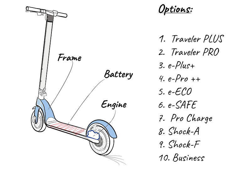
A fresh e-mobility start-up has just finished her business plan. The market for e-scooters is growing. Every year, the market expands two digits. Because more people are using it, market segmentation is extending beyond ‘driving fun’ to include segments like going to work, short city trips, going to college, and so on. There are new customer demands with each new segment: it does not have to be just for fun. There are other factors to consider, including speed, safety, and comfort. With this in mind, this startup built a minimalist-style frame that can be modified with a range of alternatives (figure 1). As a result, instead of having to create ten separate products, they can simply produce this frame and add the alternatives. Manufacturing costs fall, and so does the time to market.

Figure 1 shows the options: Option 1 and 2, having higher-speed engines. Options 3 to 6 has higher capacity batteries (3, 4), a battery that charges when braking (5), increasing it’s charging time, and (6) with a battery specially protected for all-road situations. Options 8 and 9 has special scooter frame reinforcement that aims to be a safe-guard for accidents: option 8 is in aluminum and 9 in carbon fiber. Finally, option 10 includes larger wheels with customized suspension for a more comfortable ride.

The problem

The ‘problem’ is the same as it is for many startups: cash. This is critical to launch products to market. The Mechanical Engineer manager poses a critical question to the rest of the team:

“We have enough funds to make 100 basic frames and 100 accessories. It takes three weeks to receive and adapt a new accessory. People just hate having to wait so long for this product. We need to do an initial stock, but what accessories should we purchase? Do we get ten of each?”

This is a tricky question. Accessories will conform to the final product and cannot be combined. So far, we have ten finished products to showcase. We don’t know which ones will be more successful. Our ideal condition should having more final products that we know will sell quickly, as well as a few units from those that we know would sell slowly. The earnings from the first sales can then be used to invest in new accessories, allowing our company to grow more quickly.

The marketing research

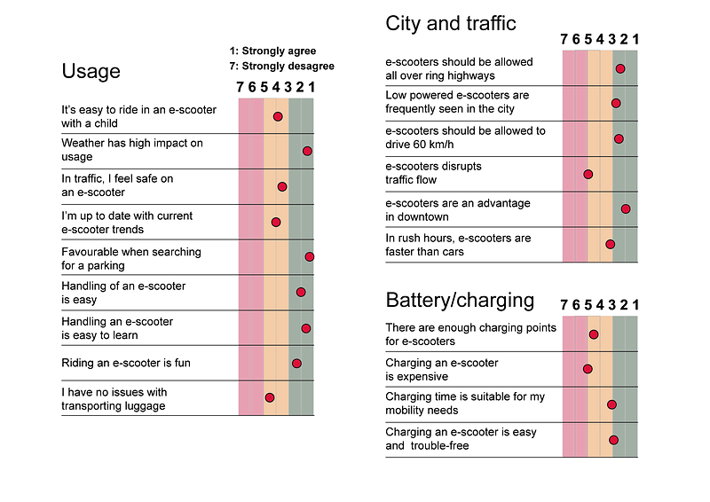
The startup team immediately begins work on a marketing research project. They also discover a report on the use of e-scooters in metropolitan areas [2]. In this article, they conduct a series of interviews with potential buyers about e-scooters. Figure 2 illustrates the results.

Multi-armed bandits in action

A bandit problem is a sequential game where player interacts with a game device. Player is often called learner and the game device is the environment. The game is played over n rounds, where n is a positive natural number called the horizon. In each round the learner first chooses an action A from a given set of actions, and the environment then reveals a reward. Armed slot-machines are the typical examples of a multi armed bandit problem. Players has to choose an arm and machine will show a price (a reward). Every time player chooses and arm is performing an action a, that is included in the set of actions represented by all alternatives the player has. For example, if slot machine has ten arms, then player has ten possible actions to choose. Actions’ sequences are registered in a history and player learns from past actions (history) in order to optimize future steps. The mapping from histories to actions is called policy (π). The policy is player’s knowledge about this environment. Player can have some prior information about the environment. This information is called environment class [3] and also true value [1] denoted as 𝑞∗(𝑎). We could say the true value of an action is the mean reward when that action is selected.

Imagine someone watching others play slot machines in a casino. During the last hour, he saw a machine that gave higher pricing than others. The remaining machines have lower prices. When the previous players have left, our player selects this machine (machine number one) since he has prior knowledge of two high prices in the last hour. Of course, this isn’t statistically significant, but it’s all information our player has.

Through repeated action selections, we want to maximize our winnings by concentrating our actions on the best choices. As we don’t know the action values with certainty, we have to estimate it. This is what the bandit algorithm does.

Exploration vs. exploitation

When the player begins the game, he uses the previously learned information (environment class or true value) to select machine number one from above example. This is referred to as exploitation, and it applies to utilizing the knowledge he already possesses. However, our player would also like to try out different levers in to get more knowledge (maybe there is something interesting over there¡). This is known as exploration. The solution to the bandits problem is to estimate the values of actions in order to use the estimates to create action selection decisions that maximize the expected total reward over some time period.

The solution to the bandits problem is to estimate the values of actions in order to use the estimates to create action selection decisions that maximize the expected total reward over some time period.

Balancing exploration and exploitation will be a fundamental calculation for our estimation. When we always exploit current knowledge to maximize immediate reward, we are using greedy action selection methods. An alternative to acting greedily all the time is to dedicate a small amount of time (with a probability ε) to exploring other alternatives. Then we are using ε-greedy action selection methods. Probability ε is the parameter that will help us to balance exploration vs. exploitation selection methods. When do we use one or another? The greedy method performed significantly worse in the long run because it often got stuck performing suboptimal actions. When we have true values with low uncertainty, it makes no sense to invest a lot of time in exploration. We can exploit the knowledge we already have. But when this true values has a high uncertainty we expect that exploiting this knowledge will not be enough so we should go exploring to maximize our winnings.

Can we solve our startup problem with multi-armed bandits?

Our startup’s challenge is one of resource allocation. We have limited resources and must manage them efficiently in order to maximize our winnings (to have more sales with the same investment). We have 10 competing possibilities (if we choose one, we can’t choose the others). Consider having a street shop where you may bring one final product (frame + accessories) per day. What option to take to the shop will be the action. A customer can come into the shop and buy the final product or not. Then you go home, and the next morning you bring another choice and repeat the same method for n time steps. Of course, we are not going to create a business and only sell one product. We are going to build a store where we will sell all of our products. However, this is a similar scenario to multi-armed bandits problem explained before. Then we can solve the startup problem with the multi-armed bandit in order to determine the best accessory selection to maximize our sales in the first hundred units batch test.

Some maths and pseudo-code

There are a number of methods for estimating the optimal action values in a multi-armed problem. We will adopt the previously described ε-greedy action selection method as well as the upper-confidence-bound action selection method. Figures four and five shows both methods.

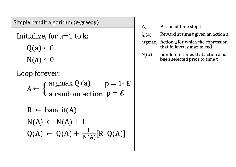
The Bandit algorithm must keep track of all rewards collected. It must estimate the average of all n rewards using this record (Qn). This can be done in the following way [1]:

where [Target-Old Estimate] is an estimation error (equal to Rn-Qn). This error is known as regret of the learner relative to a policy, and it is defined as the difference between the total total expected expected reward using policy for n rounds and the total expected reward collected by the learner over n rounds.

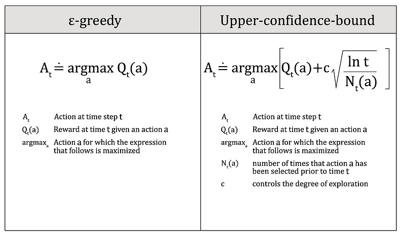
The upper-confidence-bound approach selects non-greedy actions based on their potential for being optimal, taking into account both the closeness of their estimations to being maximal, and the uncertainties in those estimates. Remember that non-greedy actions are forced to be tried at random by ε-greedy action selection methods.

Defining our problem in python

To start to solve our problem and give the best advise to this startup, we have to define the environment. The first thing we will do is to define our true values. As our time started to do, we will use the market research [2] to estimate true value.

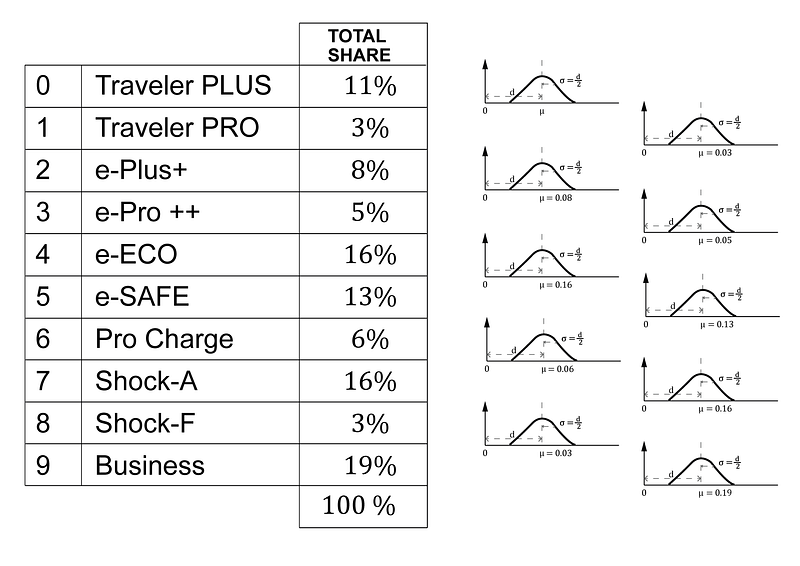
Figure 6 shows a list of all of our accessories. We will establish a market share for our sales. We’ll build a list with the condition that the sum of all market shares be 100 (or normalized to 1). Then we round out this list by assigning greater values to some options that the research says are more relevant to customers. Lower ratings are assigned to those features that appear to be less important. The entire amount is 100. This list can be normalized to sum 1. Then we have the list below, which can be produced straight in Python:

We have a lot of uncertainty on this values. Our estimation comes from some qualitative responses in market research. For including this uncertainty, we can consider that our true_values are not this values. Instead, we are going to consider them as probability distributions with 𝜇 equal to this values and 𝜎 equal to 𝜇 / 2. It is, for higher 𝜇 values we have higher 𝜎 values. We are a bit conservative so we are not pretty sure of those accessories we think are going to have more sales. For those models, we think we are going to have fewer sales; we have less uncertainty. As a rule of thumb, more sales, more uncertainty.

On these values, we have an important uncertainty. Our estimate is based on qualitative replies from market research. We can include this uncertainty by assuming that our true_values are not these values. Instead, we’ll think of them as normal distributions with 𝜇 equal to our true_values list, and 𝜎 =𝜇 / 2. It is true that for higher 𝜇 values, we also have higher 𝜎 values. We are a bit conservative, so we are unsure about the accessories we believe would sell well. We have less uncertainty for those who believe we will have fewer sales. Furthermore, we estimate larger values for the accessories (more sales). Our environment, considering this uncertainty, can be written inside a class as follows:

class BanditEnv:
    def __init__(self):
        self.size = 10
        self.means = m_size
    def step(self, action):
        assert action == int(action)
        assert 0 <= action < self.size
        reward = np.random.normal(loc=self.means[action], 
              scale=self.means[action]/2) #gaussian distribution
        return reward

Now we have to define our algorithm according figure 4:

def epsilon_greedy(env, nb_total, eps, eps_factor=1.0):
    rewards = []
    Q = np.zeros(env.size)   # shape: [n_arms]
    N = np.zeros(env.size)   # shape: [n_arms]
    for _ in range(nb_total):
        if np.random.rand() > eps:
            A = np.random.choice(np.flatnonzero(Q == Q.max())) 
        else:
            A = np.random.randint(env.size)  # explore randomly
            R = env.step(A)
            N[A] += 1   
            Q[A] += (1/N[A]) * (R - Q[A]) # incremental mean          
            eps *= eps_factor # epsilon decay
            rewards.append(R)return Q, np.array(rewards)

where env is our environment, nb_total is the number of time steps for our experiment, eps = ε and eps_factor is the decay factor for ε. The calculation will give a new list of ‘market share’ calculated after nb_total steps, together with rewards obtained with every time step.

env = BanditEnv()
nb_total=1000
epsilon = 0.1
Q, rewards = epsilon_greedy(env, nb_total= nb_total, eps=epsilon)

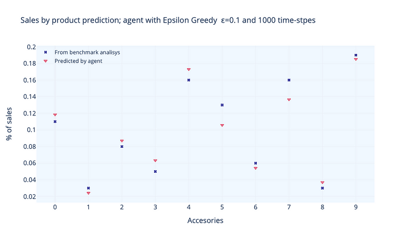
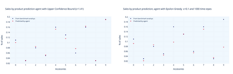
Figure 7 illustrates the findings with ε=0.1. After 1000 time steps, we may compare our true values to the calculated values. The results are pretty comparable to our initial values, with the exception of a few accessories. We can think of time-steps as every time a consumer comes into our shop and purchases an option. Controlling the exploration-exploitation balance and the time steps are important parameters for the calculation. A value of ε=0.1 indicates that the algorithm allocates 10% of its computation cost to ‘exploring’ new actions. If we increase this amount, we run the risk of the algorithm assigning too much weight to low-reward behaviors, which will have an impact on the optimization problem. Figure 8 can help us evaluate this behavior.

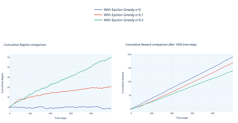
We can see that cumulative rewards and cumulative regrets must grow with time. It is critical that regret does not rise linearly (as it does with ε=0.0). We can also see that higher values (ε=0.5) have stronger regret increase than lower values (ε=0.1), and the same with rewards. We want to see a significant rise in rewards. These two metrics can be considered our agent’s performance metrics.

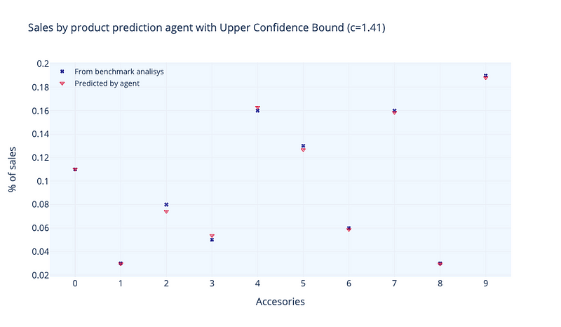
In figure 9 we can see the results obtained using Upper-confidence-bound algorithm. When using this algorithm, a typical value for c is 1.41 (√2). We see that calculated market share is very similar to our true-values. Higher the value, higher the uncertainty (higher 𝜎). So, environment uncertainty also is a topic that deeply influences the final results. If we say to our environment that we are very sure of our true values (low uncertainty), algorithm will show results very similar to ours. If we are not quite sure (high uncertainty), values can differ largely.

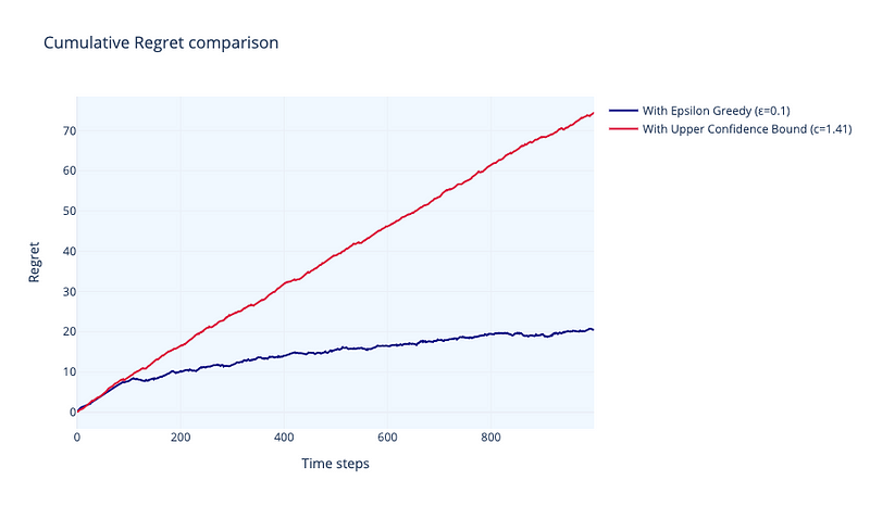
Let’s compare both algorithms. In figure 10 we can see a comparison of regret from both algorithms with time-steps. Performance of ε-greedy algorithm is clearly superior. Regret is linearly growing and, about 300 time-steps decreases its growing rate.

Environment uncertainty

We have highlighted the role of environment uncertainty in the final results of both algorithms. In the above examples we have introduced our true-values with a 𝜎 value of 𝜇/2. We are going to say to our algorithm that we are even less convinced about the values we are giving. And we will do it by choosing 𝜎 to be equal to 𝜇 (with 𝜎 = 𝜇 we are increasing uncertainty by two times). Both algorithms shows higher differences between true-values and calculated values, being ε-greedy the one where this differences are clearly higher. In figure 11 we can see how both algorithms show larger variations between true-values and calculated values, with ε-greedy clearly showing the largest differences.

Conclusions

This is the final table we can show to this startup, comparing the values we got from the market research and the calculations from our algorithms:

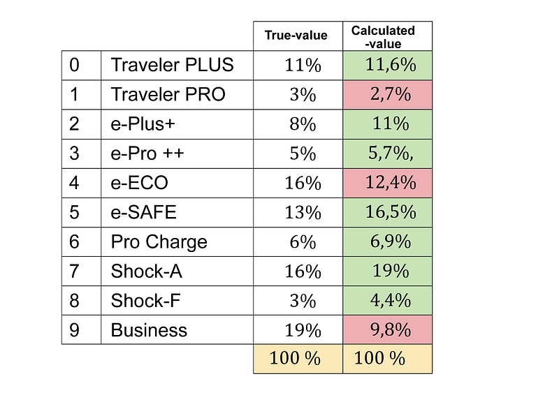
We’ve shown how a simplified version of the multi-armed bandits method may be extremely useful in solving real-world problems. Resource allocation is a type of decision-making concern that occurs frequently in most organizations. These decisions can be replicated in a variety of complexity environments. We used a very minimal setup to describe a common decision process in this post. We’ve shown how to use a multi-armed bandit algorithm to automate this decision process in order to get more accurate outcomes under uncertain conditions.

Python code

We have used numpy library for algorithm and plotly for plots. Code can be found here.

References

[1] Richard S. Sutton and Andrew G. Barto (2020), Reinforcement Learning: An Introduction. The MIT Press.

[2] Hardt, Cornelius & Bogenberger, Klaus (2018). Usage of e-Scooters in Urban Environments. Transportation Research Procedia. 37. 10.1016/j.trpro.2018.12.178.

[3] Lattimore and Csaba Szepesvári (2020). Bandit Algorithms. Cambridge University Press.