Should we already learn quantum computing?

Introduction

When it comes to quantum computing, far too many people envision something far in the future, such as traveling to Mars. However, many organizations and scientists are now devoting their time to bringing quantum mechanics closer to solving everyday problems. I’ve decided to take a tour of the various existing ecosystems and test one or more of them to see in first place, the level of complexity, second, the various ones and their applicability, and third, whether or not it has has sense to go to the qbit to solve ‘classic’ problems.

Something I learned is that you need some quantum mechanics concepts to understand why you do certain steps. Also, complex algebra is required to understand how you do these steps, as well as some computer scientist skills to know where to apply it. The good news is that you do not need to understand all of quantum physics or extremely complex algebra. To deal with it, you must be familiar with some axioms and processes that may appear counterintuitive at first.

State of the art of Quantum Computing

QC’s future is still in the realm of speculation. The prospect of a second quantum digital revolution scares as much as it excites. Many businesses have been digitalizing their operations for several years. But now are hearing that quantum computing will change (we don’t know when) everything again. With new advances in QC, ‘quantum skepticism’ is also growing. The Twitter account ‘Quantum Bullshit Detector’ (@BullshitQuantum) has begun a nice work in setting the limits of quantum technologies today and in future. They verify tech news announcing or a fictional universe where ‘qbits’ will solve every problem we can imagine, or a Mirror Universe where things go wrong. The scientific community have claimed (F. Arute et al. Nature 574, 505–510; 2019) about the use of the term quantum supremacy, inciting to use the word ‘advantage’ instead of ’supremacy’ to avoid both false illusions and misunderstandings. Scott Aaronson points out that if we can separate ourselves from the physics (which is perplexing and counterintuitive) and the “hype,” applications with quantum processors open up a new world of “real” possibilities for ML and other digital technologies. We don’t know where it will arrive, but we can see some interesting developments very close to us right now.

What industry leaders do?

“Today, the probability of bringing up quantum computing in any discussion about any computing problem is close to one.”

Chris Retford, Google Data Engineer

Google, Amazon, Facebook, IBM, and Microsoft began investing in this field over ten years ago. According to their own words, they will not be able to develop reliable quantum processors with low errors and sufficient capabilities until 2030. The largest successfully tested quantum processor known to date is Google’s Sycamore, which has 54 qubits. However, this processor is still from the “non-default-tolerant” generation, which is also referred to as “small-scale” or “near-term” to indicate that it is still in its early stages. Physicists formally defines current state of the art as NISQ (Noisy Intermediate-Scale Quantum technology) to highlight the source of the current technical problems: noise. The reader could wonder that 54 quantum bits is something limited but we have to think that in the quantum world computing capabilities grows exponentially with the number of qubits. However, the more qubits that are linked, the more difficult it is to keep their fragile states while the device is operating, and the higher the errors. Physicists believe that there is still much work to be done before quantum computers can run advanced algorithms without errors (noise-free).

Despite quantum computers are away to mainstream practical applications, tech giants like Google, Amazon, IBM or Microsoft have adapted its services platforms to offer quantum computing services. They are focusing in solving simple problems where it’s IBM Q quantum processors outperforms CPU, GPU and TFU. For example, IBM is also in the range of 50 qubits and offers the specific SDK Quiskit to operate with its quantum processors. They have developed a range of specific algorithms to work on finance or chemistry problems. They have persuaded companies such as JP Morgan and Barclays to investigate how its algorithms outperform traditional ML algorithms when it comes to predicting risks or values of financial options. The test was successful, and the financial industry is enthusiastic about its potential applications. They have also assisted manufacturers such as Mitshubishi Chemicals in simulating the mechanisms of LiO2 reactions in their batteries in order to improve this technology. CERN uses IBM Q to improve its current classification algorithms in the quest for interactions between fundamental particles. This is a short list of its SDK early adopters.

Google is concentrating its resources on hardware development. John Martinis, Google’s Chief Scientist-Quantum Hardware, heads a team that is attempting to answer some of the fundamental questions about understanding and controlling the quantum universe in order to lead the race to ‘quantum advantage’. Its approach differs from IBM’s in that it places less emphasis on real-world applications at the moment.

Microsoft has introduced the Microsoft Global Program, which is very close to IBM’s approach but partnering with important players like Honeywell or ION-Q. Azure Quantum platform provides all of the required layers to solve problems with quantum processors today. Its approach shows a very good picture of the whole ecosystem, providing solutions that are very customer-centric (in specific problems).

Introduced in 2019 at the campus of the California Institute of Technology, the Amazon AWS Center for Quantum Computing is an initiative to improve future quantum computing systems. This center offers a similar approach to Microsoft by offering a fully managed service (Amazon Braket) that allows users to begin experimenting with computers from multiple quantum hardware providers in a single place. The place is still an experimenting platform where Amazon have started to build it’s fully managed vision.

Quantum Machine Learning

“Quantum computing just become vastly simpler once you take the physics out of it.”

Scott Aaronson, University of Texas Austin

Quantum processors are focused on three quantum mechanics phenomena [4]:

• discretization,
• superposition, and
• entanglement

Discretization means that some physical variables can only have a set of possible available values. For examples electrons inside atoms shows this nature.

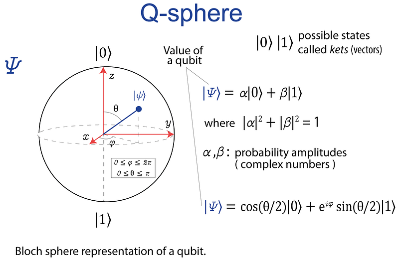
Quantum mechanics is the study of the physical states of systems, that is, all available information about these systems. According to quantum mechanics, some pairs of magnitudes cannot be measured or defined in a system at the same time. This only occurs with some magnitude pairs, specifically those that do not commute. Assume we’re looking at the location of a specific particle. Quantum mechanics tell us that, for example, a certain particle x can be in two different positions at the same time, and postulates that particle x states can be defined in both positions at the same time. This is referred to as superposition. If a particle is defined in two positions, in witch position really is? We don’t know. It is in both positions or in any of them. We don’t have any idea until we really “measure” it. And when we measure, we will find the particle in only one position (referred as well as one quantum state). Quantum mechanics postulated that if we repeat this measurement a sufficient number of times, there is a probability p that particle is in state one and a probability p’ that is in state two. Quantum mechanics is then probabilistic and predictive.

In quantum mechanics we can have two apparently separate states. But if this two states have been created under certain conditions, as a result we can not describe any of them independently from the other. We can see particles separated in space but its quantum description is global because its quantum states are entangled. The only condition is that this two particles can not interact with anything in the universe or the entanglement is lost.

Applied to quantum computing, we can operate this phenomena in the following way:

• Discretization allows us to choose systems having in a physical magnitude only two available states (0 and 1).
• We can be at state 0 or state 1 (classical computing), but also in a superposition of states 0 and 1. This is what we refer to as qubit, and has the property of concentrating the information from up two classical bits ( \(2^1\) bits) . For example, if I have a set of thousand ions with two quantum states, if these ions are in superposition, I’ll get thousand qubits; it is \(2^{1000}\) classical bits.
• If these thousand ions are entangled, I can operate over the complete set of ions. I can manipulate all these ions at the same time.The existence of entangled states is a physical fact that has important consequences for quantum computing and quantum information processing in general. In fact, without the existence of such states, quantum computers would be no more powerful than classical processors.

In a quantum computer, we enter information, we have a processing step, and we get an output. The main difference is this intermediate process is significantly different from a classic computer because it uses the three special phenomena described above. Exploiting these phenomena, we can do things that can’t be done with classical processors.

Quantum machine learning operates by manipulating states in quantum systems. We can do this manipulation representing quantum algorithms as circuit diagrams (Figure 2-a). This is an analogy coming from electronic circuits where we have an input and an output. The circuit has different components, such as resistors, transistors, or diodes, and each performs an operation. Quantum circuits work alike: they have an input and an output, have several components and each of this performs an operation. This quantum operations are based in the axioms described above.

In a complex vector space, a vector always represents the state of any quantum system (Figure 1). This is referred to as a Hilbert space. Also, any quantum system’s state is a normalized vector. Circuits enable us to perform transformations on this vector space. The quantum processor’s first step will always be to load “classical” data. In this experiment, for example, I’ll use the circuit-centric approach [1][2], in which data is encoded into the amplitudes of a superposed qubit state (Figure 1). This method is referred to as amplitude encoded quantum machine learningAnother popular method for quantum machine learning is variational algorithms (VQA) [2]. They use a classical optimizer to teach a parametrized quantum circuit how to get close to the right answer to a problem. Variational algorithms In the experiment described in [3], I’m going to combine both methodologies. This combination takes advantage of the benefits of amplitude encoding, but it is based on a variational approach [5], and it is specifically designed for small-scale quantum devices. [3] contains the complete theoretical background. There are additional resources to help you gain a deeper understanding of theoretical questions [6].

5. A basic classification task

“If small quantum information processors can create statistical patterns that are difficult to compute by a classical computer, they can also recognize patterns that are not classically recognizable.”

With this idea, I want to make an experiment using available quantum technology to perform a simple classification task. Then compare to a classical machine learning algorithm. Our dataset is a multi-class case where the target value is a non-linear combination of several features. I chose the circuit-centric approach described here [3] for two reasons:

• the current state of the art of available q-processors limits the number of qubits available,
• and this method is specific to performing classic machine learning tasks with a small number of qbits.

This approach is often referred to as Low-depth Quantum State Preparation (LDQST) [7]. LDQST reduces circuit depth (time) by introducing probabilistic quantum state preparation algorithms.

Figure 2-a shows the circuit-centric quantum classifier concept. A quantum processing unit performs inference using the model f(x,θ) = y.

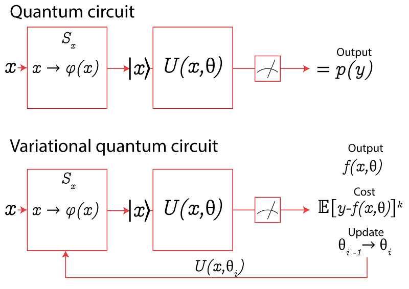
It computes a state preparation circuit \(S_x\) that encodes the input \(x\) into quantum system amplitudes, a model circuit \(U(\theta)\), and a single qubit measurement. The calculation retrieves the model’s likelihood of predicting 0 or 1, from which the binary prediction can be deduced. The classification circuit parameters θ can be learned and trained.

Four steps are involved in inference with the circuit-centric quantum classifier (Figure 2-b).

• Step 1 encodes input vectors into the n-qubit system by running a feature map from input space to feature space.
• Step 2: The quantum circuit applies a unitary transformation to the feature vector, which is analogous to one linear layer of a neural network.

In order to extract information from a quantum system, we need to perform a “measurement”. A quantum system has an infinite set of possible states, but when we make a basic measurement, we can only extract a finite amount of information. The number of outcomes is equal to the dimension of the quantum system.

• Step 3: After executing the quantum circuit, in step 3 we measure the statistics of the first qubit. This measure is interpreted as the classifier’s continuous output by adding a learnable bias term to produce the continuous output of the model (step 4).

Implementation

For implementation, I have chosen the open source IBM Qiskit library by IBM. Qiskit can be viewed as a Python library for quantum circuit execution. To run an experiment on a real quantum computer, you need to setup your IBM account first. Also, you can run it in a quantum simulator (not a real quantum processor). In our experiment, we have used a quantum simulator qsm-simulator with two qubits, and we have checked the differences using a real quantum processor from (see notebook).

import numpy as np
import seaborn as sns
from qiskit import *
from qiskit.tools.jupyter import *
import matplotlib.pyplot as plt
import pylatexenc
from scipy.optimize import minimize
from sklearn.preprocessing import Normalizer, normalize, binarize, Binarizer
from sklearn.model_selection import train_test_split
from sklearn.preprocessing import StandardScaler, MinMaxScaler
from sklearn.decomposition import PCA, KernelPCA, LatentDirichletAllocation
import pandas as pd


# For using a quantum simulator:
backend = BasicAer.get_backend('qasm_simulator') 

# For using a real quantum processor:
# Using a real quantum processors from IBM
IBMQIBMQ.save_account('xxxxxxxxxxxxxxxxxxxxxxxxxxxxxxxxxxxxxxxxxxxxxxxxxxxxxxxxxxxxxxxxxxxxxxxxxxxxxxxxxxxxxxxxxxxxxxxxxxxxxxxxxxxxxxxxxxxxxxxxxxxxxxxxxx')
provider = IBMQ.load_account()

"""You can check in IBM site the cues in different backend processors and choose the ones with lower cues to speed up your work""" 
backend = provider.backends.ibmq_london

We are going to perform a classification task in a dataset with  \(N=19\) features, including the target feature. As a preparation step, we will perform a dimensionality reduction with PCA to  \(N=2\) components as we want to use a 2-qubit simulator. Data preparation and dimensionality reduction are done with Scikitlearn library. The complete code can be found here.

Step 1. Encoding data

Quantum algorithms that are only polynomials in the number n of qubits can perform computations on 2n amplitudes.

Entanglement makes it possible to create a complete 2n dimensional complex vector space to do our computations in, using just n physical qubits.

If these 2n amplitudes are used to encode the data, one can therefore process data inputs in poly-logarithmic time. Entanglement makes it possible to create a complete 2n dimensional complex vector space to do our computations in, using just n physical qubits. So, given a unitary vector of dimension four, we extract five angles with the function get_angles. These angles will be used as arguments for encoding our data in quantum a circuit (in Figure 3, \(R\) refers to rotation angle in \(Y\)).

# Arguments for encoding quantum circuit

def get_angles(x):
    beta0 = 2 * np.arcsin(np.sqrt(x[1]) ** 2 / np.sqrt(x[0] ** 2 + x[1] ** 2 + 1e-12))
    beta1 = 2 * np.arcsin(np.sqrt(x[3]) ** 2 / np.sqrt(x[2] ** 2 + x[3] ** 2 + 1e-12))
    beta2 = 2 * np.arcsin(
        np.sqrt(x[2] ** 2 + x[3] ** 2) / np.sqrt(x[0] ** 2 + x[1] ** 2 + x[2] ** 2 + x[3] ** 2)
    )
    return np.array([beta2, -beta1 / 2, beta1 / 2, -beta0 / 2, beta0 / 2])

# Angles obtained:
First features sample:[ 0.81034968, -0., 0., -1.22809981, .22809981]

The circuit preparation, including angles, is the following.

# State preparation circuit
def statepreparation(a, circuit, target):   # a:angle
    a = 2*a
    circuit.ry(a[0], target[0])         # rotation angle on y
    circuit.cx(target[0], target[1])    # CNOT gate
    circuit.ry(a[1], target[1])         # rotation angle on y
    circuit.cx(target[0], target[1])    # CNOT gate
    circuit.ry(a[2], target[1])         # rotation angle on y
    circuit.x(target[0])                # x value
    circuit.cx(target[0], target[1])    # CNOT gate
    circuit.ry(a[3], target[1])         # rotation angle on y
    circuit.cx(target[0], target[1])    # CNOT gate
    circuit.ry(a[4], target[1])         # rotation angle on y
    circuit.x(target[0])                # x value
    return circuit

x = X_norm[0]
ang = get_angles(x)
q = QuantumRegister(2)
c = ClassicalRegister(1)
circuit = QuantumCircuit(q, c)
circuit = statepreparation(ang, circuit, [0,1])
circuit.draw(output='mpl')  #for plotting the circuit diagram

The schematic for our state preparation circuit will look as follows:

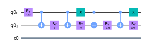
where a 2x2 matrix is the representation of X-gate. Both X-gates are on a 0 qubit. R are the rotation angles (five in total), and connectors are CNOT gates (Figure 4).

Step 2. Model circuit.

The circuit has several stacked blocks, which can be called layers, to make an analogy with neural networks. A layer is composed of a general parameterized unitary gate applied to both qubits. Below we can see the final circuit, including state preparation, model circuit, and measurement.

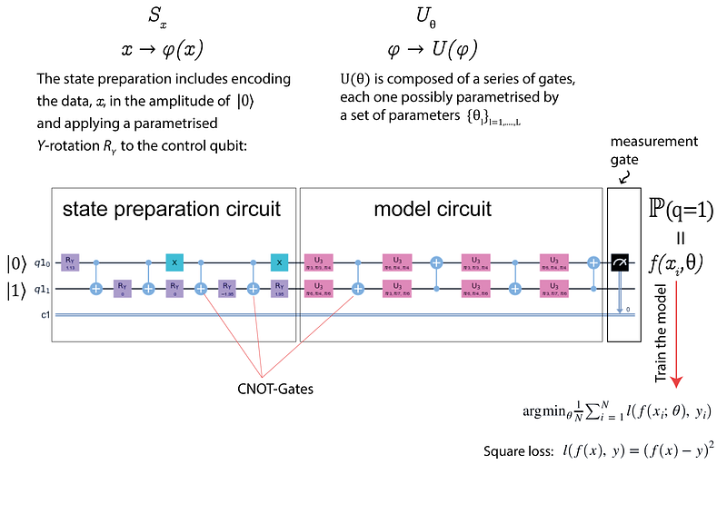
We apply the operator to the feature state \(U(\theta)\), where \(\theta_i\) are trainable parameters (see Figure 4). The following code executes the model circuit:

def execute_circuit(
          params, 
          angles=None, 
          x=None, 
          use_angles=True, 
          bias=0, 
shots=1000
):

    if not use_angles:
        angles = get_angles(x)  
        
    q = QuantumRegister(2)
    c = ClassicalRegister(1)
    circuit = QuantumCircuit(q,c)
    circuit = statepreparation(angles, circuit, [0,1])
    circuit = create_circuit(params, circuit, [0,1])
    circuit.measure(0,c)
    result = execute(circuit, backend, shots=shots).result()
    counts = result.get_counts(circuit)
    result=np.zeros(2)
    
    for key in counts:
        result[int(key,2)]=counts[key]
        
    result/=shots
    return result[1] + bias

execute_circuit(params, ang, bias=0.02)

Step 3. Training the model

We have to find a predictor \(f\) to estimate \(y\) given a new value of \(x\). We will train a model with the training input by finding the parameters \(\theta\) that will minimize a loss, \(l\) (Figure 4). In our example, \(f\) will return the probability of being labeled \(l\).

Step 4. Measurements and results

After performing the measurement, we have got the following results (Figure 5).

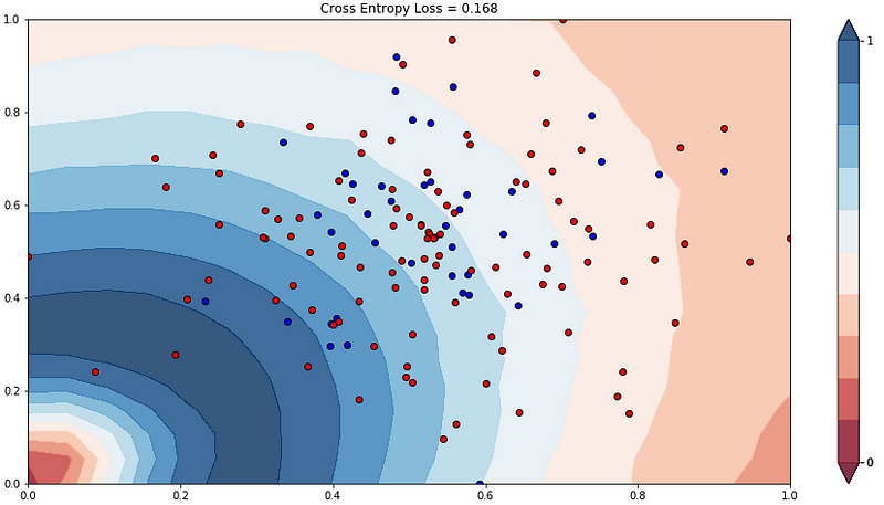
5.2 Results and benchmark

We used cross-entropy loss, or log loss, to calculate the accuracy of our model, which measures the performance of a classification model whose output is a probability value between 0 and 1. As the predicted probability diverges from the current label, cross-entropy loss increases. Figure 5 shows the end result. In addition, we carried out the same classification task using various standard algorithms to compare our results (Figure 6).

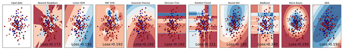
As we can see, our result is slightly better than the best result got with the Nearest Neighbors algorithm. In any case, the probability that model guesses for the correct class is lower than 0.8 . Reader may think that the effort to use quantum algorithms is too high. I personally do. But I have to consider the complete process where I have reduced dataset dimensionality with standard ML algorithms in order to use only 2 qbits. The idea was to use a low-depth quantum state preparation method. Though results are still promising.

Conclusions

“Once you are familiar with the axioms of quantum mechanics, superposition or entanglement appears to you as a natural thing.”

J.I Cirac, Max-Planck-Institut für Quantenoptik

Okay, so it's important for you to get to know some basic principles of quantum mechanics. Otherwise, you might find yourself getting stuck in all the steps needed to create quantum algorithms. To be able to write these algorithms, however, some knowledge of complex algebra is required. Unlike neural networks, the difficulty here is in understanding why you do what you do. The challenge with neural networks is understanding what they have done. With all of this, the advances have been significant. It’s not just about the number of qubits; it’s about realizing that the results of quantum algorithms can provide a new perspective on pattern recognition. Neglecting issues such as speed and computation power, quantum computing may be interesting today, despite its limitations.

References

[1] Kosuke Mitarai, Makoto Negoro, Masahiro Kitagawa, Keisuke Fujii (2018) ‘Quantum Circuit Learning’, Phys. Rev. A 98, 032309.

[2] Jacob Biamonte, Peter Wittek, Nicola Pancotti, Patrick Rebentrost, Nathan Wiebe, Seth Lloyd (2017), ‘Quantum Machine Learning’, Nature 549, 195–202 .

[3] Maria Schuld, Alex Bocharov, Krysta Svore, Nathan Wiebe, (2020) ‘Circuit-centric quantum classifiers’, Phys. Rev. A 101, 032308.

[4] Müller-Kirsten, H. J. W. (2006). Introduction to Quantum Mechanics: Schrödinger Equation and Path Integral. US: World Scientific. p. 14. ISBN 978-981-2566911.

[5] Macaluso A., Clissa L., Lodi S., Sartori C. (2020) A Variational Algorithm for Quantum Neural Networks. In: Krzhizhanovskaya V. et al. (eds) Computational Science — ICCS 2020. ICCS 2020. Lecture Notes in Computer Science, vol 12142. Springer, Cham. https://doi.org/10.1007/978-3-030-50433-5_45

[6] Giuliano Benenti , Giulio Casati and Giuliano Strini (2004). Principles of Quantum Computation and Information, Default Book Series.

[7] Xiao-Ming Zhang, Man-Hong Yung, Xiao Yuan, (2021) ‘Low-depth Quantum State Preparation’, arXiv:2102.07533

Disclaimer: This post originally appeared in 2019.

More fundamentals in:

• IBM’s Qisqit : https://qiskit.org/textbook/what-is-quantum.html
• Quantum Algorithm Implementations for Beginners, Abhijith J. and Adetokunbo Adedoyin and John Ambrosiano and Petr Anisimov and Andreas Bärtschi and William Casper and Gopinath Chennupati and Carleton Coffrin and Hristo Djidjev and David Gunter and Satish Karra and Nathan Lemons and Shizeng Lin and Alexander Malyzhenkov and David Mascarenas and Susan Mniszewski and Balu Nadiga and Daniel O’Malley and Diane Oyen and Scott Pakin and Lakshman Prasad and Randy Roberts and Phillip Romero and Nandakishore Santhi and Nikolai Sinitsyn and Pieter J. Swart and James G. Wendelberger and Boram Yoon and Richard Zamora and Wei Zhu and Stephan Eidenbenz and Patrick J. Coles and Marc Vuffray and Andrey Y. Lokhov. 2020, 1804.03719, arXivcs.ET