Untangling AI systems: How Physics Can Help Us Understand Neural Networks

What if we could open up an AI system and find a well-organized factory of components that work together? The article explores a new approach that combines two powerful concepts: sparse neural circuits and physics-inspired mathematics. By combining these different areas, we could find new approaches for analyzing and building AI systems. While neural networks appear to be elusive black boxes, researchers have uncovered something engrossing: they contain interpretable "circuits" that function similarly to machine components. Let me explain in simple terms.

Neural Circuits

What if, instead of trying to understand an entire neural network at once, we could examine it piece by piece, just as biologists study individual cells and neural pathways? This approach, inspired by neurology and cellular biology, was pioneered by Chris Olah back in 2018, offering a more thorough way to understand neural networks.

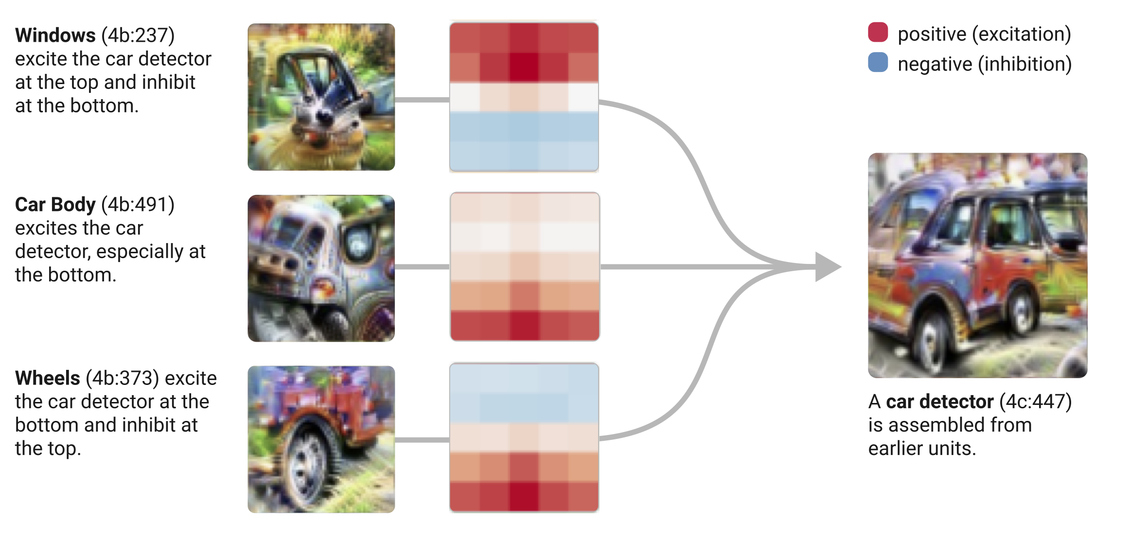
Think about how we recognize a dog in a picture. Our brain processes different features: the curve of the ears, the texture of the fur, the roundness of the eyes. Neural networks work similarly, but with a crucial challenge that Olah identified: their neurons are "polysemantic" – they respond to multiple, often unrelated features at once. Like a complex recipe, neural networks combine these features with specific "weights" – imagine mixing 80% of feature A with 50% of feature B and 30% of feature C. These weights act as glue, connecting lower-level features (like curves and textures) into higher-level ones (like dog faces). As Olah noted, "weights connect features, forming circuits." These circuits can also be rigorously studied and understood.

Think about a factory

Imagine walking into a modern factory. You can see several machines working together: one selecting items, another assembling them, and a third performing quality checks. Each machine performs a distinct role, yet they all work together to create the final product. Neural networks operate in remarkably similar ways. Instead of functioning as a single unit, neural networks consist of smaller components known as circuits, each of which carries out a specific function. Let's dig deeper into this analogy.

• Component Specialization

Just as a factory's quality control station may have specialized sensors for identifying specific flaws (size, color, texture), brain circuits create specialized detectors for specific features. While some circuits identify edges, others recognize patterns, and still others recognize more complex combinations, each circuit, like manufacturing machinery, has a specific function.

• Assembly Line Process

A factory's different stations process raw materials before transforming them into finished goods. Similarly, in neural networks, raw input (such as pixels in a picture) passes through circuits that process progressively complex features. Similar to how diverse manufacturing processes transform raw metal into a car part, simple edge detection may combine with additional traits to ultimately recognize a whole object.

• Interconnected Systems

Machines in a factory don't work alone; they "talk" to each other using computer systems, sensors, and conveyor belts. The output of one machine is the input for another. Weights connect neural circuits in the same way that a factory's quality control system may send products back for rework.

We can learn about AI systems by recognizing and identifying their circuits, much as we can understand a factory by studying what each machine performs. And, much as a factory manager can improve production by adjusting individual machines, knowing neural circuits may enable us to fine-tune AI systems with remarkable precision.

Making AI Circuits Practical and Powerful

Imagine trying to optimize our factory but discovering a particular challenge: each worker or machine is simultaneously performing multiple unrelated tasks. One station might be both painting parts and checking quality, while another both packages products and manages inventory. This is exactly the challenge we face with traditional neural networks—their components (neurons) handle multiple, overlapping tasks, a phenomenon known as "superposition" \(^{[1]}\). To understand why this happens, consider a factory forced to operate with fewer workers than needed. To maintain productivity, each worker takes on multiple roles, making it difficult to understand or improve any single process. Similarly, neural networks develop "polysemantic neurons—individual components that juggle multiple features because they have fewer neurons than features they need to represent.

Superposition

The basic idea behind superposition is that neural networks "want to represent more features than they have neurons," thus they use a property of high-dimensional spaces to simulate a model with many more neurons.

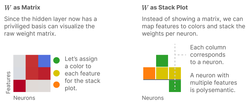
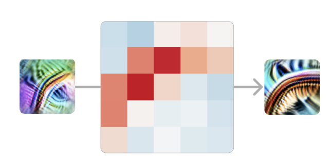
Looking at the figure above, the right side (Stack Plot) shows that one neuron (represented by a column) contains multiple colored blocks, each representing a different feature. As a result, the neuron is "polysemantic"—it has several meanings. We can magine each column as a worker in our factory. The colored blocks represent different tasks or responsibilities. Just as it would be challenging to understand or modify a worker's performance when they're handling multiple overlapping duties, these polysemantic neurons make it difficult to interpret or enhance specific functions in our AI systems.

Consider a worker who performs different tasks at the same time rather than focusing on one. Just as it can be challenging to understand the exact nature of the worker's responsibility, superposition complicates the interpretation of a specific neuron's actions in the network, as it manages multiple features or concepts simultaneously. This is why traditional neural networks are sometimes referred to as "black boxes"; their internal workings are difficult to understand because individual components (neurons) do not have unique, single purposes but rather a combination of multiple functions.

Sparse Feature Circuits

Specialized autoencoders in the sparse feature circuits approach \(^{[2]}\) have the advantage of separating features, making each machine part clearly distinct. Then we can actually see what each part does independently. We call it "feature disentanglement." It generates individual interpretable semantic concepts that are easy to understand and measure, as well as enabling efficient attribution of causal effects. 

Traditional circuits might recognize "dogs" but mix up ears, tails, and fur. Sparse circuits clearly separate features like "pointy ears," "wagging tail," and "furry texture." With the traditional circuits approach, changing one element often resulted in the disruption of others, akin to unraveling a sweater by pulling one thread. Sparse circuits allow modifying specific features without affecting others. We can improve how an AI recognizes product defects without affecting its color perception.

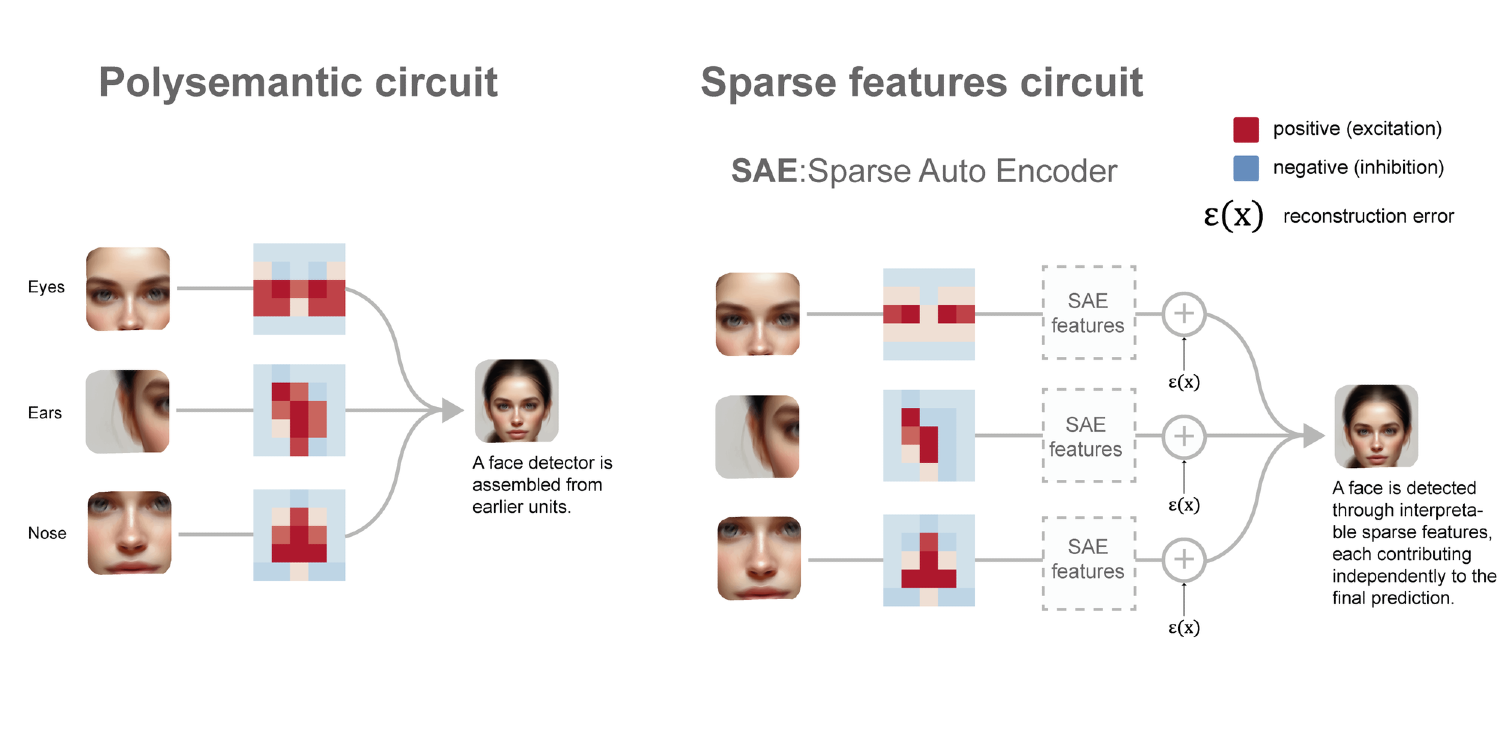
Think of reorganizing our factory so each worker or machine handles just one specific task. Through specialized techniques (like sparse autoencoders), we could separate these tangled features into distinct, interpretable components. Instead of having one circuit handling both "pointy ears" and "wagging tails," we could have dedicated circuits for each feature.

The Physics Behind AI Circuits

Just as factory layouts follow principles of efficiency and natural workflow, we can use concepts from physics (specifically Hamiltonian mechanics) to guide how these separated features should interact. This approach doesn't just separate features - it helps us understand the natural "flow" of information through the system.

When we think of a modern factory, we imagine an automated system in which every machine and component works in sync. AI systems, like well-tuned factories, contain internal machinery that needs to work smoothly and consistently. Physics, particularly Hamiltonian mechanics, provides us with important capabilities for understanding and improving AI circuits. Consider monitoring a factory's performance. You can check how much energy each machine needs and how smoothly materials flow between stations. We're also interested in how part changes affect the whole system and which manufacturing paths are most efficient.

Similarly, with AI circuits, we need to calculate how much "energy" each feature requires and analyze how information flows between features. Understanding how changes propagate through the system can help us identify the most efficient processing paths. To accomplish this, we can use Hamiltonian mechanics—a commonly used approach in physics for analyzing complex systems that have multiple interacting elements. Physicists use this approach to study the movement of planets or the interaction of particles, and we can apply it to understand the interplay of features in AI circuits. Initially, scientists developed this method to study energy-efficient mechanical systems \(^{[3][4][5][6][7][8][9]}\). This approach doesn't just separate features - it helps us understand the natural "flow" of information through the system.

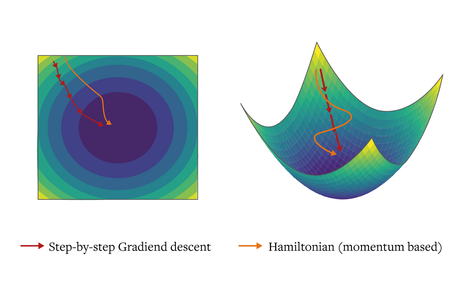
The Hamiltonian framework provides a principled way to discover and analyze circuits by treating them as dynamical systems in phase space. To understand this, think back to our factory analogy: imagine tracking a production line not just by its current state (where products are, what each machine is doing), but also by how quickly and efficiently things are changing (production rates, energy usage, workflow momentum).

In physics, this complete description of a system's state and its changes is called phase space. Just as we might plot both a pendulum's position and its velocity to fully understand its motion, we can describe our AI system using both its current configuration and how it's changing. This dual perspective is captured mathematically in what's known as the Hamiltonian. The key equation is \(H(q,p)=T(p)-V(q) \), where \(q \) represents the current state of the model's parameters, \(p \) is the change in parameters (momentum), and \(T(p)\), \(V(q)\) are the "kinetic energy" representing the cost of changing states, and the "potential energy" representing how well the current state performs.

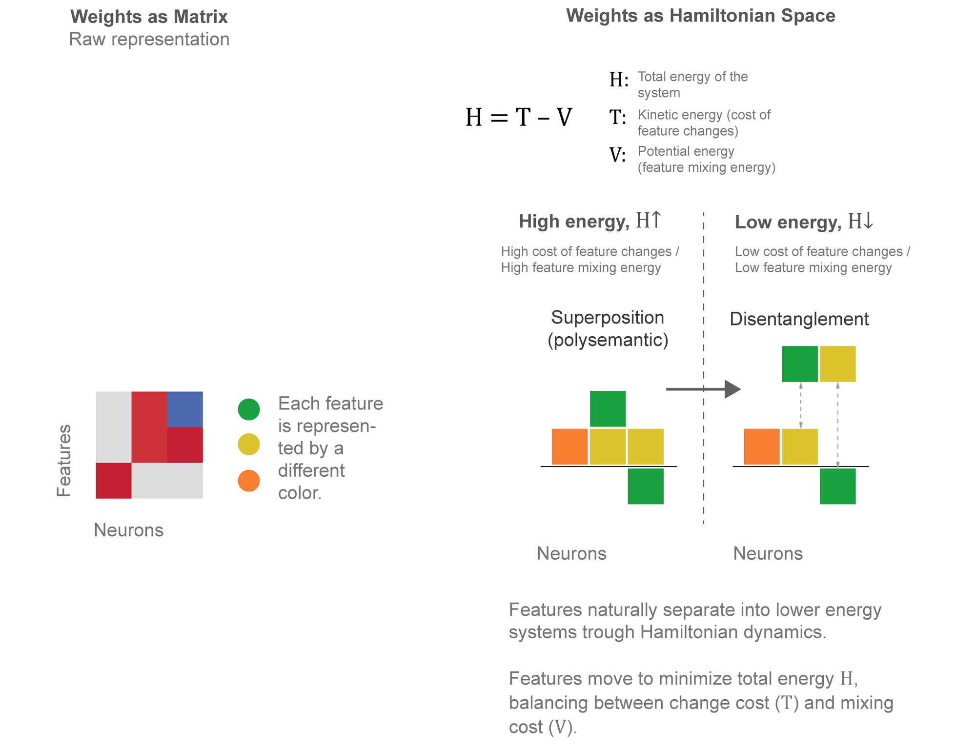
The beauty of Hamiltonian mechanics is its ability to break down complex systems into two simple components: potential energy (how stable or effective a state is) and kinetic energy (how things change over time) \(^1\). In our AI circuits, potential energy helps us understand how well features achieve their tasks, whereas kinetic energy shows us how features adapt and change as they process information. By balancing these two properties, just as a pendulum balances height and velocity, we can discover the most significant features and then figure out how they should interact.

The Hamiltonian \(H\) provides a natural optimization objective. Features that contribute to task performance lower potential energy \(V(q)\). Changes in feature activations contribute to kinetic energy \(T(p)\). The Hamiltonian system naturally finds circuits that balance performance with stability. The Hamiltonian approach can be used to efficiently compute indirect effects using linear approximations using symplectic geometry. It provides a principled way to measure feature importance while enabling systematic discovery of circuits without prior hypotheses.

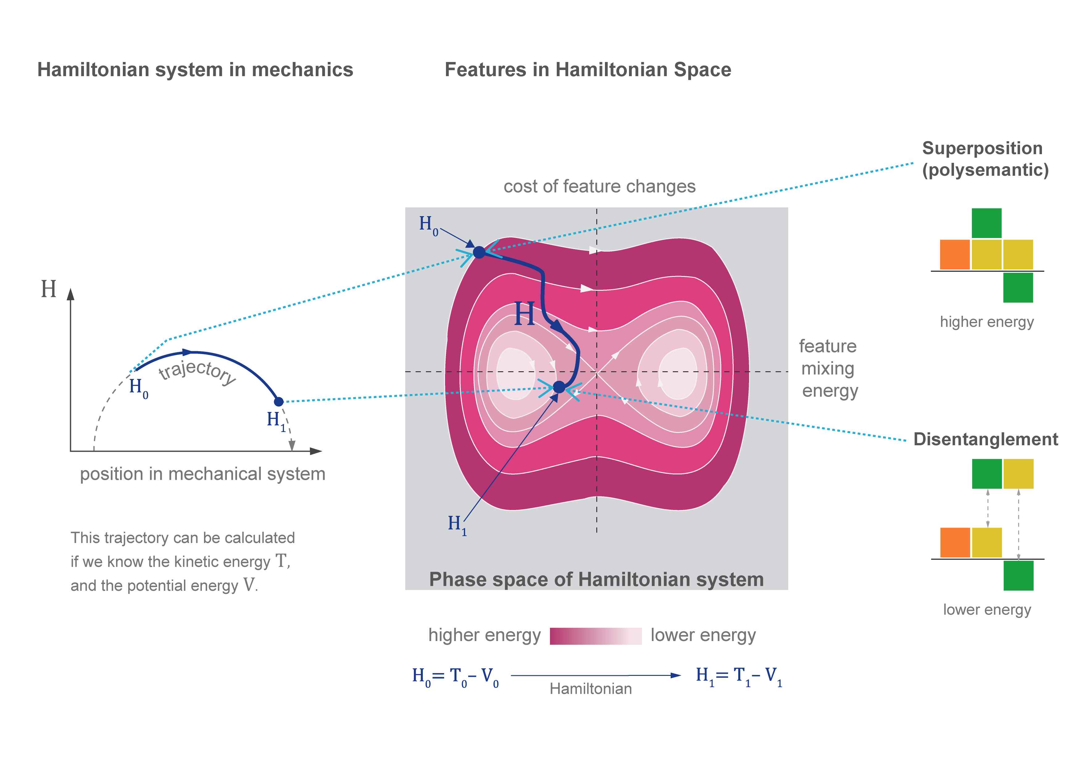
Think of the above figure as a "before and after" snapshot of our reorganized factory. The left side represents our initial "polysemantic state" - imagine a chaotic factory floor where each worker handles multiple, overlapping tasks. Each vertical column represents a neuron (or worker), and the colored regions show different features or tasks they're handling simultaneously. The overlapping colors visualize how these features are tangled together, making it difficult to modify or understand any single function. The right side shows our target "disentangled state"—the same factory after applying our Hamiltonian-guided reorganization. Notice how the colors have separated into distinct bands. Just as we might rearrange our factory so each station handles one specific task, this disentangled state shows neurons that have become specialized. Each feature has found its natural place, making the system more interpretable and manageable. The curved arrows between the states represent the Hamiltonian dynamics-guided gradual transition. Like water naturally flowing downhill, our physics-inspired approach helps features find their optimal separation without forcing them into predetermined positions. This natural evolution helps maintain the system's functionality while achieving better organization.

We can think about complete energy \(H\) functions as a compass, guiding us to the right features. When \(H\) remains constant (conserved), it allows us to identify which features are really important, equivalent to how a pendulum preserves its entire energy when translating between height and motion.
We use a mathematical structure called symplectic geometry \(^2\) to ensure that when features change, their important connections remain preserved \(^{[10][11]}\). It's similar to having a map that preserves distances and angles; even if things move, the important connections remain unaltered. As features naturally move toward their optimal states (momentum based approach \(^3\)), it becomes clear which features cause or impact others. Consider water moving downhill: it automatically picks the most efficient paths, and by observing its flow, we may learn how different sections of the landscape interact.

Combining the Approaches: The Best of Both Worlds

Conventional circuits allow for the combination (superposition) of features. Sparse circuits can help separate features, but they require a plan of action. Hamiltonian physics addresses the natural mechanism of separation.
Sparse circuits identify features, but Hamiltonian physics explains how to separate them via energy minimization. This is similar to having a map (sparse circuits) and a compass (Hamiltonian dynamics). 

This combination enables sparse circuits to discover interpretable features, while Hamiltonian dynamics guides them to naturally separate. As a result of this combination, features separate more quickly and consistently. Also, Sparse circuits allow us to target certain features, and Hamiltonian physics assures that modifications follow natural routes. Thus, the combination allows us to change features without affecting others. Finally, sparse circuits provide comprehensible feature components, and Hamiltonian conservation principles ensure that features remain separated once disentangled.

For example, if we want to prevent gender bias from a classifier, the combined approach shows its effectiveness: sparse circuits first allow us to identify which specific features are related to bias based on gender, while Hamiltonian physics gives a natural mechanism to separate these biased features from the positive ones. Instead of blindly altering the system, we may use Hamiltonian dynamics' energy-minimizing paths to gradually remove biased features while retaining the classifier's basic functionality. Think of untying a knot carefully by following its natural form instead of forcefully separating ropes; at last, there is a neat split that has no ripple effect throughout the system.

Looking Forward

We have explored the idea of combining Hamiltonian dynamics and sparse feature circuits, which opens up new possibilities but also raises important questions that need our attention. Consider how this approach could expand into much larger language models; will the same concepts apply to models with billions or trillions of parameters? Addressing the computational cost of training sparse autoencoders remains a major concern.
However, the potential benefits are significant. Consider AI systems whose actions we can genuinely understand and safely change, allowing us to surgically remove undesired biases or boost specific capabilities without unexpected consequences. The physics-inspired approach provides a theoretical foundation for this, but we must consider how we might make these tools more accessible to practitioners who do not have substantial physics backgrounds.

We've seen how Hamiltonian dynamics can help with feature separation, but there's a lot more to explore. Could other physics principles such as quantum mechanics, statistical mechanics, or field theories provide more insights? We encourage readers to look into these possibilities and perhaps explore them in their own work. What physical concepts can you use for your specific AI challenges?

There are also practical questions to address. While this method is promising, how will it perform in real-world applications with noisy data and complex tasks? We need to conduct research on the robustness and dependability of this method in various contexts.

We are still in the process of developing the combination of physics and AI interpretability. What other physical concepts can we use to better understand and develop AI systems? Could this strategy result in entirely distinct AI architectures inspired by physical systems? 

References

[1] Elhage, et al., "Toy Models of Superposition", Transformer Circuits Thread, 2022.

[2] Marks, S., Rager, C., Michaud, E. J., Belinkov, Y., Bau, D., & Mueller, A. (2024). Sparse feature circuits: Discovering and editing interpretable causal graphs in language models. arXiv preprint arXiv:2403.19647.

[3] De León, M., & Rodrigues, P. R. (2011). Generalized Classical Mechanics and Field Theory: a geometrica approach of Lagrangian and Hamiltonian formalisms involving higher order derivatives . Elsevier.

[4] Easton, R. W. (1993). Introduction to Hamiltonian dynamical systems and the N-body problem (KR Meyerand GR Hall). SIAM Review , 35 (4), 659.

[5] Leimkuhler, B., & Reich, S. (2004). Simulating hamiltonian dynamics (Issue 14). Cambridge university press.

[6] Marsden, J. E., & Ratiu, T. S. (2013). Introduction to mechanics and symmetry: a basic exposition of classical mechanical sys tems (Vol. 17). Springer Science & Business Media.

[7] Easton, R. W. (1993). Introduction to Hamiltonian dynamical systems and the N-body problem (KR Meyerand GR Hall). SIAM Review , 35 (4), 659.

[8] Marin, J. (2024). Optimizing AI Reasoning: A Hamiltonian Dynamics Approach to Multi-Hop Question Answering. ArXiv Preprint ArXiv:2410.04415 .

[9] Marín, J. (2024). Hamiltonian Neural Networks for Robust Out-of-Time Credit Scoring. arXiv preprint arXiv:2410.10182.

[10] Forest, E., & Ruth, R. D. (1990). Fourth-order symplectic integration. Physica D: Nonlinear Phenomena , 43 (1), 105–117.

[11] Marsden, J. E., & West, M. (2001). Discrete mechanics and variational integrators. Acta Numerica , 10 , 357–514.

Footnotes

\(^1\) One of the simplest examples of Hamiltonian system is a frictionless pendulum. In a frictionless pendulum, the total energy is the sum of potential, and kinetic energy is conserved through its evolution.

\(^2\) Symplectic structures are fundamental geometric objects in differential geometry and classical mechanics and support Hamilton's equations of motion by explaining the connection between position and momentum in physical systems. In simple terms, symplectic structures are specific rules that define how things move in physics, similar to an equation for motion. Poincaré’s Theorem states that any solution to a Hamiltonian system is a symplectic flow, and it can also be shown that any symplectic flow corresponds locally to an appropriate Hamiltonian system.

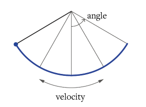
The frictionless pendulum is one of basic forms of a symplectic space.Velocity and angle are the two components that describe the movements of a pendulum. We can map this in a 2D space as a trajectory.

\(^3\) Momentum based approach translates to the algorithm being able to "roll past" small local minima in the loss landscape,
potentially finding better global or local minima that simple gradient descent might miss. The conservation of the Hamiltonian (total energy) ensures that the system maintains this exploratory behavior throughout the optimization process, unlike in some other methods where the exploration gradually decreases.